Temporal evaluation and projections of meteorological droughts in the Greater Lake Malawi Basin, Southeast Africa
 Lucy Mtilatila
 Axel Bronstert
 Klaus Vormoor1
- 1Institute for Environmental Science and Geography, Potsdam University, Potsdam, Germany
- 2Department of Climate Change and Meteorological Services, Ministry of Natural Resources and Climate Change, Blantyre, Malawi
The study examined the potential future changes of drought characteristics in the Greater Lake Malawi Basin in Southeast Africa. This region strongly depends on water resources to generate electricity and food. Future projections (considering both moderate and high emission scenarios) of temperature and precipitation from an ensemble of 16 bias-corrected climate model combinations were blended with a scenario-neutral response surface approach to analyses changes in: (i) the meteorological conditions, (ii) the meteorological water balance, and (iii) selected drought characteristics such as drought intensity, drought months, and drought events, which were derived from the Standardized Precipitation and Evapotranspiration Index. Changes were analyzed for a near-term (2021–2050) and far-term period (2071–2100) with reference to 1976–2005. The effect of bias-correction (i.e., empirical quantile mapping) on the ability of the climate model ensemble to reproduce observed drought characteristics as compared to raw climate projections was also investigated. Results suggest that the bias-correction improves the climate models in terms of reproducing temperature and precipitation statistics but not drought characteristics. Still, despite the differences in the internal structures and uncertainties that exist among the climate models, they all agree on an increase of meteorological droughts in the future in terms of higher drought intensity and longer events. Drought intensity is projected to increase between +25 and +50% during 2021–2050 and between +131 and +388% during 2071–2100. This translates into +3 to +5, and +7 to +8 more drought months per year during both periods, respectively. With longer lasting drought events, the number of drought events decreases. Projected droughts based on the high emission scenario are 1.7 times more severe than droughts based on the moderate scenario. That means that droughts in this region will likely become more severe in the coming decades. Despite the inherent high uncertainties of climate projections, the results provide a basis in planning and (water-)managing activities for climate change adaptation measures in Malawi. This is of particular relevance for water management issues referring hydro power generation and food production, both for rain-fed and irrigated agriculture.
Introduction
Droughts are a major hydrological hazard in many regions of the planet affecting several sectors of societies, such as food production, municipal water supply and hydropower generation. Due to increasing demand for food, water resources and energy, droughts have received ever increasing attention in the last decades and innovative methods of drought assessment and analysis (e.g., Stahl and Demuth, 1999; Vogel et al., 2021) and prediction and modeling (e.g., Krol et al., 2006; de Araujo and Bronstert, 2016; Pilz et al., 2019; Adnan et al., 2021) have been presented. Though less documented in science literature, droughts are also common in southern Africa and their frequencies and severities are increasing (Masih et al., 2014). This situation has not spared Malawi, which relies heavily on natural water resources of the Lake Malawi and Shire River Basins. Lake Malawi has many water inlets but only one outlet, the Shire River in the South where about 98% of the country's hydropower production takes place (Taulo et al., 2015). Runoff into the Shire River largely relies on outflow from Lake Malawi, which is mainly a function of lake level. However, the lake level has decreased by ~1.0 m over the period 1970–2013 (Mtilatila et al., 2020a). This has created low flows on Shire River and affected the production of electricity (ESCOM, n.d.). The occurrence of drought events also affects agricultural production. Coulibaly et al. (2015) estimated that 53.3% of crop failure in Malawi is due to climatic factors including droughts, floods and high temperatures, and yet agriculture contributes almost 28–30% of Malawi's Gross Domestic Product (GDP) (GOM, 2019). Therefore, the combined direct effects of floods and droughts affect Malawi's economy by reducing the annual GDP by 1.7% (Pauw et al., 2011).
According to records from the Department of Disaster Management Affairs in Malawi, there have been ten drought events since 1975 on record eight of which were major. The most severe droughts occurred in 1992 and 2015 and affected almost 7 million and 6.7 million people, respectively. These events may be referred to as agricultural droughts since the effects are linked to agricultural production, and their extent/magnitude is based on the size of the food insecure population. However, according to Spinoni et al. (2020), agricultural drought is defined as soil moisture deficit that leads to crop failure. Mtilatila et al. (2020a) studied meteorological droughts in Lake Malawi and Upper Shire River basins based on the standardized precipitation and evapotranspiration index (SPEI) and the standardized precipitation index (SPI). They came up with eight meteorological drought events between 1970 and 2013. The majority of these events lasted for more than a year and the most severe event occurred from 1992 to 1996 (Mtilatila et al., 2020a). Regionally, these events were linked to droughts that were experienced in most of the South African countries, which have generally shown an increase in the frequency of drought events from the 1980s onwards (Rouault and Richard, 2005). The meteorological droughts often trigger hydrological droughts in the Lake Malawi Basin with a delay of more than 24 months due to the attenuation effect of the lake (Mtilatila et al., 2020b). A hydrological drought in this regard is considered for lake levels below 474.1 masl developed in reference to the 1970–2013 period. Therefore, during 1970–2013 only one hydrological drought was identified. This, however, lasted for 101 months from June 1994 to October 2002. During this drought event, the lake level dropped by 0.9 m on average (Mtilatila et al., 2020a).
There is a link between observed climate change and drought occurrences in Malawi: statistically significant increasing trends in temperature (0.8°C over 40 years) and mostly insignificant decreasing trends in precipitation conditions (Mtilatila et al., 2020a) agree with increasing trends in drought conditions (Ngongondo et al., 2011, 2015; Mtilatila et al., 2020b). The temperature increase is enhancing potential evapotranspiration (PET) (Ngongondo et al., 2015). Therefore, droughts identified based on the SPEI tend to be even more severe, last longer and cover a larger geographical extent than droughts identified by SPI (Mtilatila et al., 2020a). Compared to 1976–2013, climate projections indicate future temperature increases of 0.98–2.1 and 1.8–5°C between 2021–2050 and 2071–2100, respectively, based on the Representative Concentration Pathway (RCP) 4.5 and 8.5 scenarios (Mtilatila et al., 2020b). This provides an indicator of increasing severity of future droughts, which may even be enhanced if the temperature increases are combined with decreases in rainfall. In this regard, however, future precipitation is subject to a greater uncertainty, in terms of both the extent and direction of changes (Kusangaya et al., 2014). But still, the potential impacts of future climate changes (temperature and rainfall changes) on drought conditions in Malawi have not been quantified.
Usually, the impacts of climate change on environmental systems are investigated against the background of scenario-based climate projections. General Circulation Models (GCMs) are used to estimate future changes in climate component systems and ocean circulation by means of emission scenarios for greenhouse gases and aerosol concentrations (Déqué, 2007). However, these models are at low spatial resolutions which often do not fit well with the impact scale, and the uncertainty that originates from the GCMs is high (e.g., Warnatzsch and Raey, 2018; Wu et al., 2021). To address this problem, Regional Climate Models (RCMs) are applied to dynamically downscale the GCMs to higher spatial resolutions. Nevertheless, when using GCMs as boundary conditions, errors from the GCMs are often transferred to the domain of the RCMs such that they may require further correction (Déqué, 2007; Themeßl et al., 2012). For example, Warnatzsch and Raey (2018) found that GCM–RCMs underestimated precipitation in all the seasons and the correlation between the observations and models did not exceed ±0.57 for monthly rainfall in Malawi. Though the models captured the rainfall trend, they were underestimating the slope and the inter-annual fluctuations compared to the observed dataset. Many models failed at matching observed drought episodes identified based on the SPI. Thus, statistical approaches are often applied to relate the results of GCM–RCMs to the statistical characteristics of meteorological observation data at the local or regional scale (e.g., Wilby and Wigley, 1997; Hundecha et al., 2016). Based on an ensemble of bias-corrected GCM–RCM combinations, potential impacts of climate change on drought characteristics (here based on the SPEI) can be estimated (e.g., Johnson and Sharma, 2015; Aryal and Zhu, 2017).
However, sensitivity of droughts toward rainfall and temperature changes requires a different approach. So alternatively to the “top-down” approach described above, scenario-neutral “bottom-up” approaches can be applied to assess the impacts of climate change on specific target variables (e.g., Prudhomme et al., 2010; Fronzek et al., 2011; Hirschi et al., 2011). Such approaches assess the sensitivity of a target variable (here the SPEI) to systematic changes in climate variables (here, temperature and precipitation). That is, observed climate data are systematically perturbed and the response (i.e., impact on the SPEI) of a certain combination of systematically perturbed temperature and precipitation time series is plotted as one pixel on a two-dimensional domain: the so-called “response surface”. However, at least in this simple version, such bottom-up approach neglects likely changes in the temporal sequencing of climate data (e.g., annual, seasonal, day-to-day variability). which may, however highly influence the occurrence and severity of hydrological extremes like droughts.
Therefore, the aim of this study is to examine the development of future drought characteristics in the Greater Lake Malawi Basin (GLMB) under climate change. The study, combines bias-corrected GCM–RCM simulations and projections with a scenario-neutral response surface approach as described in Vormoor et al. (2017) to analyse future meteorological droughts. With reference to 1976–2005, we seek to establish how well the 16 GCM–RCM combinations are able to simulate drought incidents and their characteristics including the number of detected events, their duration, and their intensity as compared to observation data. We also analyse the benefits of applying the bias-correction (i.e., empirical quantile mapping) for the representation of drought characteristics by the GCM–RCM ensemble over this period. In addition, the sensitivity of drought characteristics toward the changes in temperature and precipitation is conducted based on scenario-neutral response surfaces which also incorporates changes in the temporal structure of temperature and precipitation time series as they are projected by the GCM–RCM ensemble. The following specific research questions are addressed by this study:
(1) How reliable are (bias-corrected) climate models in simulating meteorological drought characteristics in the Greater Lake Malawi Basin?
(2) As climate is expected to change in the future, what are the expected changes in future drought characteristics like their intensity, duration and number of occurrences as compared to the recent past in this region?
Study area and data
Study area
The study is looking at the combined Lake Malawi and Shire Basins which is referred to as the Greater Lake Malawi Basin (GLMB). Malawi is a land-locked country located in south-eastern Africa (Figure 1). It shares borders with Mozambique to the South, Southwest and Southeast, Zambia to the northwest and Tanzania to the North and Northeast. The climate of Malawi is predominantly warm and wet from October to April, with mean temperatures varying roughly between 26 and 28°C and monthly rainfall of above 200 mm. It is generally cooler and drier in winter (May–September), with monthly rainfall below 20 mm and mean temperatures between 21 and 25°C.
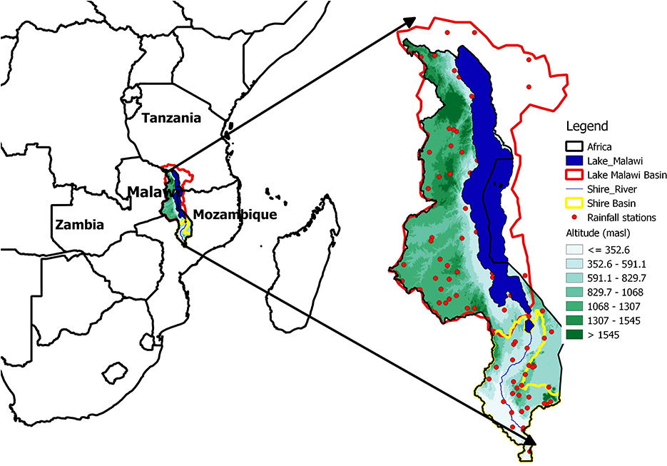
Figure 1. The study area, the Greater Lake Malawi Basin (Lake Malawi and Shire River Basins) in south-east Africa.
In terms of size, Malawi covers 118,484 km2, and in 2018, 20.4% of the area was covered by water bodies, 48% by agricultural land, 18.9% by forest and the remaining 12.6% by built-up area, barren land and other wooden areas (Source: https://knoema.com/atlas/Malawi/topics/Land-Use/Area/Surface-area). The population (currently almost 18 million people) is increasing at the rate of 2.9% per year (National Statistical Office, 2018) which adds pressure on the natural resources by increasing land under development and agriculture, hence increasing deforestation (Palamuleni et al., 2011). For example, in the Upper Shire River Basin, agricultural land increased by 18% from 1989 to 2002 (Palamuleni et al., 2011), while forest cover in the Lake Malawi Basin decreased from 64% in 1967 to 51% in 1990s (Calder et al., 1995). In 2018, the population was almost four times that of 1966 (National Statistical Office, 2018) and 86% of Malawi's population was employed in the agricultural sector in 2013 (Nyekanyeka, 2013).
Data
We used the observed gridded daily rainfall dataset that was used by Mtilatila et al. (2020b). The gridded data were generated from station data obtained from the Department of Climate Change and Meteorological Services (DCCMS) in Malawi, which was complemented by a 0.5° gridded rainfall product provided by the Global Precipitation Climatology Center (GPCC) (Schneider et al., 2018) to cover Tanzanian and Mozambiquan areas for rainfall. Daily temperature data were obtained from the Climatic Research Unit (CRU) at the University of East Anglia (Osborn and Jones, 2014). The Inverse Distance Weighting (IDW) method by Shepard (1968) was used to grid data into 0.5° to match the resolution of the GCMs. In this study, the gridded observations-based products are used as a reference and for bias-correcting 16 GCM–RCMs combinations provided by the Coordinated Regional Climate Downscaling Experiment (CORDEX) Africa (accessed at https://cordex.org/data−access/esgf/). The GCM–RCMs have a spatial resolution of 0.44° and provide daily simulations and projections, respectively, for the periods 1976–2005, 2021–2050, and 2071–2100. In this study, the RCP 4.5 and 8.5 scenarios are considered for the future climate projections to account for the high uncertainty of models in capturing rainfall in the study area (Warnatzsch and Raey, 2018). Table 1 shows the GCM–RCM combinations considered in this study.
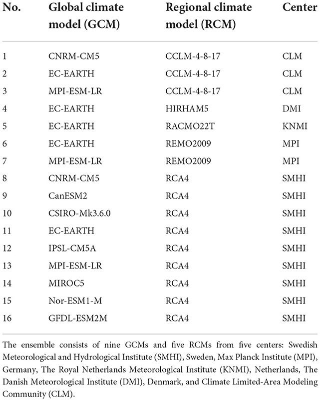
Table 1. GCM–RCM combinations from CORDEX Africa used in the study.
Methods
Drought analysis
Droughts in the GLMB are estimated based on the SPEI, which is a commonly used index to describe meteorological droughts (Vicente-Serrano et al., 2010). The estimation of the SPEI is based on the meteorological water balance (MWB), i.e., the difference between precipitation and PET. Evapotranspiration can be estimated as reference, potential or actual. The reference evapotranspiration assumes the well-watered grass surface, while the PET is based on the open water surface. In this study PET is adopted as is indicated by Vicente-Serrano et al. (2010). PET is estimated using the Thonthwaite equation (Thornthwaite, 1948), which requires only temperature as measured input, and as such is an advantage in areas where data are scarce. The distribution function of the water balance determined from the precipitation and temperature is transformed into a standard normal distribution. The SPEI then quantifies the water excess and deficits over a certain time period, as the SPEI represents the number of standard deviations by which a certain water balance estimate deviates from the long-term mean:
where xi is the MWB estimate over a given time scale, here 12 months as recommended by Mtilatila et al. (2020a), and and σ are the mean and standard deviation of the MWB, respectively (Vicente-Serrano et al., 2010). For the definition of drought characteristics, we adopted the McKee et al. (1993) classification based on SPEI instead of SPI. Droughts are defined in four categories: mild droughts (0 ≥ SPEI > −1.0), moderate droughts (−1.0 ≥ SPEI > −1.5), severe droughts (−1.5 ≥ SPEI > −2.0), and extreme droughts (SPEI ≤ −2.0). However, since the WMO (2012) characterizes mild droughts as near-normal, we neglected this category during the onset of the drought. Consequently, a drought event starts when the SPEI ≤ −1 and ends when the SPEI turns positive, and this period is referred to as drought duration in months. The total drought months (DM) and drought events (DE) are the total number of months during which the drought occurred and the total number of times droughts occurred during a 30-year period, respectively. Finally, drought intensity (DI) is the minimum SPEI value during drought duration (Dayal et al., 2017).
Empirical quantile mapping (EQM)
Future drought characteristics can be analyzed based on temperature and precipitation projections from dynamic climate models like GCMs (e.g., Haile et al., 2020) or RCMs (Tomaszkiewicz, 2021). Due to limited descriptions of the atmospheric process and rather coarse spatial resolutions the output of such models need some further statistical downscaling and/or bias correction (e.g., Bronstert et al., 2007). In this study, we applied empirical quantile mapping (EQM) to adjust biased RCM outputs to observations. This method has become popular (e.g., Piani et al., 2010; Themeßl et al., 2012; Johnson and Sharma, 2015; Osuch et al., 2017; Shrestha et al., 2020; Enayati et al., 2021), as it seeks for a transfer function to adjust the quantiles of the GCM–RCMs (xm) to those of the observed data (xo; here, gridded observations for temperature and precipitation). The method can be expressed as:
where Fm is the empirical cumulative distribution function (eCDF) of xm and is the inverse eCDF corresponding to xo (Piani et al., 2010), The transfer function identified for the current climate conditions is then applied to also adjust the future projections by the GCM–RCMs, assuming that the function is stationary and the shortcomings of the GCM–RCMs are the same for the future period. The bias correction is applied to the daily values at the individual grid points for each climate model. EQM has proved to bias-correct daily rainfall better than parametric and theoretical distribution based methods (Enayati et al., 2021). We then evaluate the performance of the raw and bias-corrected GCM–RCM combinations in terms of their ability to represent drought characteristics during the reference period (1976–2005).
Climate change impacts on drought characteristics
The potential future impacts of climate change on drought characteristics at the basin scale have been investigated by means of response surfaces. In a two-dimensional domain, response surfaces display the changes in long-term mean drought characteristics when the climatological input data (precipitation and temperature) are systematically perturbed linearly as:
Observed climate data (To(i) and Po(i)) for the reference period 1976–2005 is linearly and uniformly scaled at daily time steps, i, within a user-defined range of possible future changes given by the perturbation factors Xt and Xp for temperature (additive) and rainfall (multiplicative), respectively. Temperature is scaled in +0.5°C increments up to +5°C as compared to temperatures of the reference period, leading to eleven (11) different perturbations. Precipitation is scaled in ±5% increments within the range from −35 to +10% as compared to precipitation during the reference period, resulting in ten (10) model realizations. The perturbed time series of temperature and rainfall are applied in Equation 1 to obtain the SPEI for each of all possible combinations of perturbed input data series (11 × 10 = 110 realizations). Based on these SPEI series, changes in MWB and drought parameters (DE, DI, and DM) are derived. For a specific combination of perturbed time series, the mean change as compared to the reference period is plotted as one realization (i.e., one pixel) within the 11 × 10 domain of the response surface. The climate signals from the bias-corrected GCM–RCMs are then overlaid over the response surfaces to provide an illustration of their specific future projections including their uncertainties (i.e., range of the projections) (Vormoor et al., 2017; Mtilatila et al., 2020b).
However, the linear scaling of observed temperatures and rainfall neglects possible modifications of the temporal structures (e.g., sequences of dry/wet spells) due to climate change, as it is the case with the delta method of statistical downscaling (Sunyer et al., 2012). To overcome this issue, we also perturbed future projections of the 16 GCM–RCMs after having removed their mean climate change signal. That is, temperature and rainfall of the bias-corrected RCP8.5 scenario for the period 2071–2100 is first leveled to the observed data (i.e., removing the mean projected change signal—in magnitude) and then systematically perturbed as shown in Equations 3, 4 (see Vormoor et al., 2017 for details). This way, we preserve changes in the temporal structure as projected by the climate models.
Again, the MWB and drought parameters are estimated from the individual SPEI series resulting from the perturbed time series. In total, we generated 17 response surfaces (16 GCM–RCMs and one observed dataset) based on 1,870 perturbed times series (1obs + 16 GCM–RCM × 11Xt × 10Xp). If the changes in temporal structures of temperature and rainfall have no influence on droughts, then the response surfaces generated by perturbed GCM–RCM data and observed data are expected to be alike. In this study, we illustrate two response surfaces for each target variable: one shows the mean of the 17 individual response surfaces, and the second one summarizes the differences between the 17 response surfaces as given by the coefficient of variation (CV) for DE and DM, or the standard deviation (SD) for DI and MWB. The larger the CV or SD, the larger is the influence of the temporal structure on the water balance or a specific drought parameter.
Results
The results section is subdivided into two parts. The verification of temperature, rainfall, MWB and meteorological drought characteristics as represented by the 16 GCM–RCM combinations using the historical period of 1976–2005 is presented in Section Performance of GCM–RCMs. This is followed by changes in the future MWB and drought characteristics in Section Projected drought characteristics.
Performance of GCM–RCMs
Precipitation and temperature
The Taylor diagrams (Taylor, 2001) comprising Pearson correlations (r), standard deviation and centered root mean square errors (RMSE) are used to verify the 16 GCM–RCMs against observations for rainfall and temperature. To determine the potential improvement contributed by EQM, both raw and bias-corrected daily rainfall and temperature are presented in Figures 2A,B. Since the generation of drought characteristics is done at monthly scales, the verification of monthly rainfall and temperature is also included (Figures 2C,D). Not only does the Taylor diagram provide the opportunity to compare models with observations, but the models can also be compared with one another.
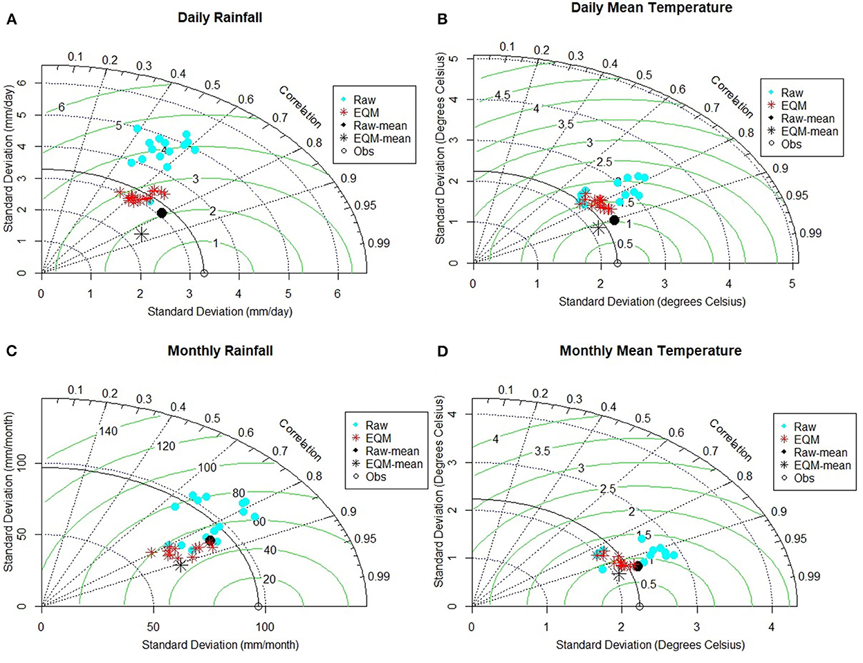
Figure 2. Taylor diagrams of (A) daily rainfall, (B) daily mean temperature, (C) monthly rainfall, and (D) monthly mean temperature. Cyan is for the uncorrected (raw) model outputs, while red is the bias-corrected model outputs. Black shows ensemble means, where • is for uncorrected outputs while* is for the bias-corrected dataset. O Represents the observed (reference) dataset. The Pearson correlation which is shown by the azimuth from 0 to 90° is significant at the 0.05 significance level. The centered root mean square error (RMSE) is proportional to the distance from the reference point on the x-axis (green lines) and is in mm/day or mm/month or degrees Celsius for daily rainfall, monthly rainfall and temperature respectively. The standard deviation is proportional to the radial distance from the reference point.
The ensemble members of the raw dataset have a bias that ranges from −25 to +21% for daily rainfall, hence the need to conduct bias correction. For daily rainfall (Figure 2A), the standard deviation of the observed daily rainfall is 3.3 mm, while all the uncorrected raw models except one show larger standard deviations. The deviation of the raw dataset ranges from 3.1 to 5.0 mm. After the bias correction, the dispersion of values in the dataset is reduced as the standard deviation range shifts to between 2.9 and 3.5 mm. The improvement introduced by EQM is also observed with the Person correlation coefficient between the observed and GCM–RCM ensemble members. The correlation improves from between 0.39–0.7 (raw ensemble members) and 0.53–0.71 (EQM ensemble members). Similarly, the root mean square error (RMSE) improves from between 2.6–4.8 and 2.6–3.1 mm per day. Considering the ensemble mean, the RMSE improves from 2.1 to 1.8 mm, and the correlation coefficient improves from 0.79 to 0.85. At the monthly time scale (Figure 2C), the skill of the EQM ensemble improves considerably, as the correlation is in the range of 0.66–0.87 (0.86 for the ensemble mean) and 0.79–0.88 (0.91 for the ensemble mean) for uncorrected and bias-corrected ensemble members, respectively.
The bias of daily mean temperature is less than rainfall, as it ranges from −6 to +11% for the raw ensemble members. The correlations are similar for both datasets which range from 0.7 to 0.84 (raw data) and from 0.72 to 0.85 (EQM data) (Figure 2B). Again, the ensemble mean correlation between the observations and the models are also similar, at 0.91. The standard deviations for both raw and corrected model outputs are near the reference point. However, the RMSE for the ensemble mean slightly improves from 1.1 (raw) to 0.9°C (EQM). Looking at the raw ensemble members, their standard deviations are greater than those of the observations, while the bias-corrected values are mostly around the observed standard deviation of 2.2°C. At the monthly time scale (Figure 2D), the standard deviations of temperature for the ensemble members also remain around 2.2°C, while the uncorrected members range from 1.9 to 2.9°C. The correlation coefficients and RMSE show similar patterns as at the daily time scale.
In summary, EQM improves the skill of the GCM–RCM ensemble by reducing the spread and magnitude of ensemble members. Most models represent the temperature of the region better than rainfall. Aggregating individual ensemble members into ensemble means as well as aggregating from daily to monthly time scales improves the statistical measures significantly.
Meteorological water balance (MWB), standardized precipitation and evapotranspiration (SPEI) and drought characteristics
To illustrate the effectiveness of EQM, the deviations in the MWB as estimated from the raw and bias-corrected climate simulations and compared to observed data for the reference period are also assessed (Figure 3A). In addition, the deviations of the SPEI, DE, DI, and DM are also evaluated (Figures 3B–E).
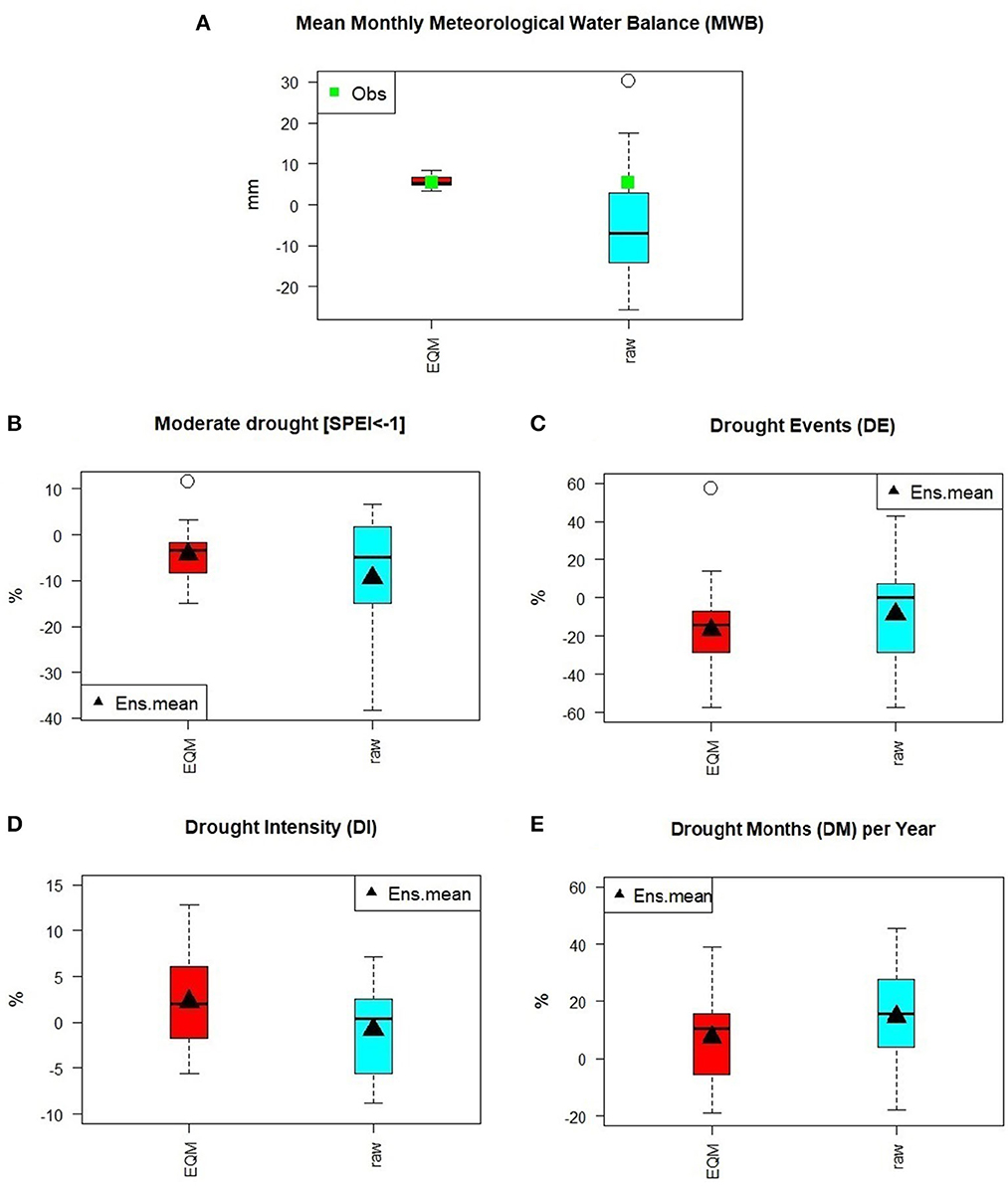
Figure 3. Bias assessment of (A) monthly mean meteorological water balance (rainfall minus PET, in mm/month), (B) standardized precipitation and evapotranspiration index (SPEI) for moderate drought (SPEI <−1), (C) drought events (DE), (D) drought intensity (DI), and (E) drought months (DM) per year in the GLMB.
MWB
The observed MWB mean is +5.5 mm, and in Figure 3A, the benefit of EQM becomes the clearest, as it corrects the water balance bias from the inter-quartile range (IQR) of between −13.4 and +2.4 mm, (ensemble mean: −3.9 mm) to between +4.8 and +6.8 mm (IQR) (ensemble mean: +5.6). The bias correction has managed to correct all the models from negative to positive MWB and closer to observed MWB values.
SPEI
Figure 3B shows the deviation of the SPEI for moderate drought events (SPEI ≤ −1). For the raw dataset, the bias ranges from −14.6 to +1.3% (IQR), and after bias correction the deviation is reduced and counts from −7.9 to −2.1% (IQR). The deviation of the ensemble mean improves from −9.4% for the raw dataset to −4.4% for the bias-corrected dataset (Figure 3B).
Drought characteristics
The deviation in the drought parameters DE, DI, and DM are shown in Figures 3C–E. The smallest deviation for both the raw and bias-corrected datasets is found for DI, Figure 3D (mean raw: −0.8% vs. mean EQM: +2.2%). The size of the ensemble distribution is similar but the EQM ensemble shows slightly larger values. For DM (Figure 3E), the range in the deviation of the raw and EQM ensembles is also similar, though based on the IQR, the EQM range has smaller deviations than raw values [EQM: −3.3 to +15.6% (IQR) vs. raw: +6.4 to +26.7% (IQR)]. However, the mean deviation of the EQM ensemble (+7%) is considerably smaller than the raw ensemble (+14%). Less influence of EQM bias correction is noted for the estimation of DE as the deviation of the raw dataset ranges from −28.6 to +3.6% (IQR) while the deviations of the EQM ensemble range from −28.6 to −10.7% (IQR) (Figure 3C).
To sum up, analogous to the improvement in rainfall, EQM considerably improves the estimation of the MWB from the GCM–RCM ensemble for the reference period. However, the effect of EQM on the estimated drought parameters is comparably small and does not necessarily lead to an improved representation of drought characteristics for the reference period.
Projected drought characteristics
Standardized precipitation and evapotranspiration index (SPEI)
Figure 4 presents the SPEI time series of the 16 GCM–RCMs and their ensemble means for the period 1976–2005 (historical period), 2021–2050 (near-term period), and 2071–2100 (far-term period) using the bias-corrected datasets. The SPEI during the historical period shows high uncertainty and variations among the individual models. As a result, the ensemble mean of the models rarely goes beyond −1 and +1, and it is clearly noticed that the ensemble members are poorly representing the observed SPEI (RED graph) during the historical period. Over time, though, the SPEI decreases which indicates an increase in DI from the historical period to the near- and far-term periods in Malawi. The wet episodes noted during the historical period become fewer and fewer in the future, as dry conditions become more prominent. The increase in drought during 2021–2050 is similar for both RCP4.5 and RCP8.5, but the mean intensity of RCP8.5 is 21% more than that of RCP4.5. During 2071–2100, the SPEI based on RCP4.5 stabilizes, while the SPEI based on RCP8.5 constantly keeps on decreasing. It is also noted with many ensemble members that they have one continuous drought episode during the entire period of 2071–2100. The model uncertainty (spread of models) is large, which starts during the historical period and increases over time. The SPEI based on RCP8.5 shows greater uncertainty than based on RCP4.5, and the mean intensity of the SPEI based on RCP8.5 is 171% larger than that based on RCP4.5 during this period.
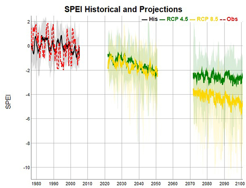
Figure 4. The standardized precipitation and evapotranspiration index (SPEI) series for observations and the 16 bias-corrected GCM–RCM combinations and associated ensemble means for (i) the historical period 1976–2005, gray-ensemble members, black-ensemble mean, and red-observations. (ii) 2021–2050 and 2071–2100 future periods. Green-RCP4.5 and yellow-RCP8.5.
Projected changes in drought characteristics
The previous sections have illustrated the limited ability of the GCM–RCM ensemble (both raw and bias-corrected) to represent the observed meteorological water balance and drought characteristics for the reference period. This also limits the credibility of the GCM–RCM ensemble in projecting potential future changes. Therefore, we opted for the response surface approach as described in Section 3.3 to illustrate the sensitivity of droughts to systematic changes in temperature and precipitation (Figure 5). The future projections of temperature and precipitation of the GCM–RCMs are overlaid on the response surfaces to illustrate the ensemble uncertainty. The summary of the GCM–RCMs is also represented in Table 2.
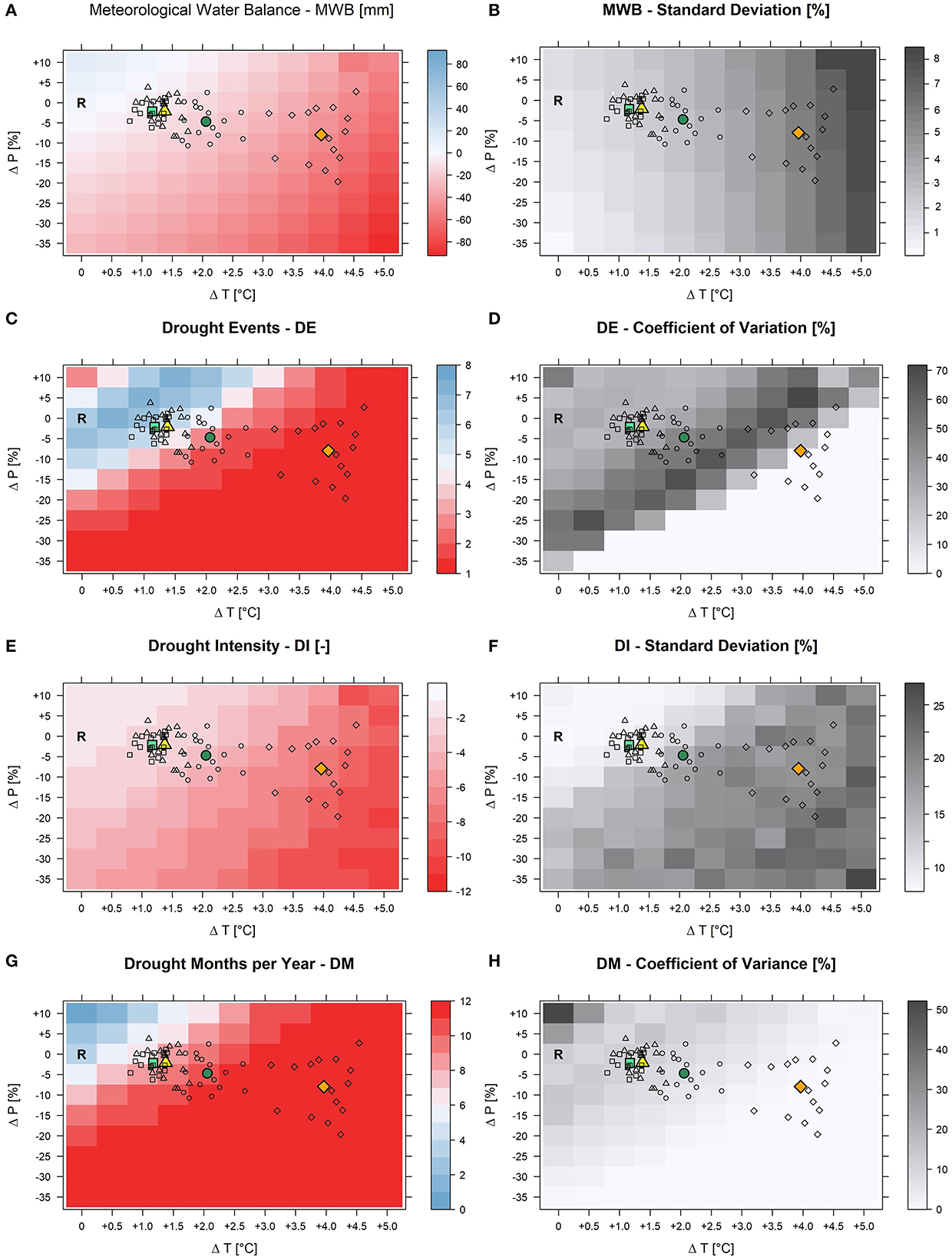
Figure 5. Response surfaces for mean meteorological water balance-MWB [first row-(A,B)], mean drought events-DE [second row-(C,D)], mean drought intensity-DI [third row-(E,F)] and drought months-DM per year [fourth row-(G,H)] at the aggregated scale of GLMB. The response surfaces are produced using systematically perturbed precipitation (y-axis) and temperature (x-axis) data as inputs. The points added on the surfaces reflect climate change signals as projected by 16 GCM–RCM combinations. The different symbols refer to different periods and scenarios (rectangle/circle: RCP4.5 2021–2050/2071–2100; triangles/diamonds: RCP8.5 2021–2050/2071–2100 for the bias-corrected datasets. Thick colored symbols are the mean of the climate model ensemble for the bias-corrected datasets for the respective periods and scenarios: light-green/dark-green for RCP4.5 2021–2050/2071–2100; yellow/orange for RCP8.5 2021–2050/2071–2100. Response surfaces in the left column show the mean of 17 individual response surfaces (16 generated based on leveled GCM–RCMs plus 1 based on scaling observed time series). Panels to the right show the standard deviations and coefficient of variation, respectively, of the 17 individual response surfaces. “R” marks the mean of each drought parameter for the reference period, i.e., no scaling.
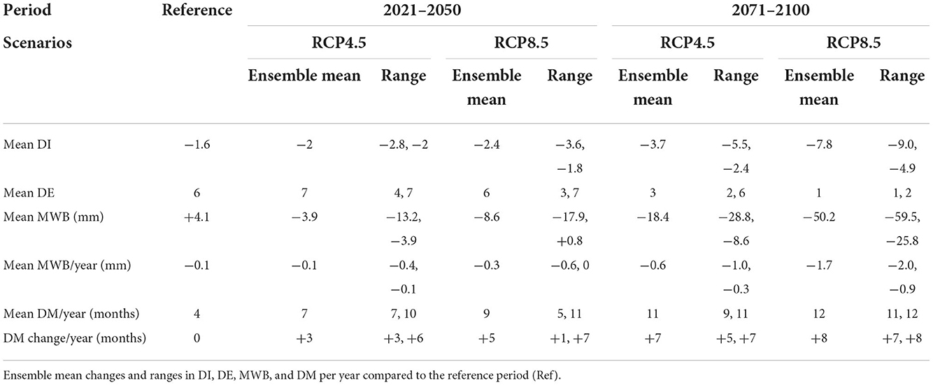
Table 2. Summary of GCM–RCM results.
Meteorological water balance (MWB)
The mean MWB is sensitive to both temperature and rainfall changes (Figure 5A) as the estimates decrease with both increasing temperature and decreasing precipitation. The MWB at the reference point, R (ΔP = 0%; ΔT = 0°C) is ~+4.1 mm, indicating that the rainfall amount is greater than evapotranspiration (water surplus). However, for the most extreme combination of scaling (ΔP = −35%; ΔT = +5°C), the MWB is negative (~-92.3 mm) implying that evapotranspiration clearly exceeds rainfall. It is also found that already an increase of just 1°C in temperature (ΔP = 0%; ΔT = 1°C) changes the water balance to −3.9 mm implying that evapotranspiration becomes higher than rainfall in the area. Similarly, the change in rainfall of ±5% (ΔP = ±5%; ΔT = 0°C) changes the MWB to +8.8/−0.5 mm.
Considering the GCM–RCM ensembles, most of the models suggest future MWB between −3.9 and −13.2/+0.8 and −17.9 mm during 2021–2050 for RCP4.5/RCP8.5. These estimates reflect a decrease in MWB between −195 and −422%/−80 and −537% respectively. During 2071–2100 and for RCP4.5, the water balance is in the range of −8.6 to −28.8 mm, which reflects a decrease of −320 to −802%. For RCP8.5 on the other hand the water balance is from −25.8 to −59.5 mm, reflecting a decrease of −729 to −1,551%. The ensemble mean changes for the different periods and RCPs are −3.9 (−195%) and −18.4 (−549%) (RCP4.5 2021–2050 and 2071–2100), and −8.6 (−310%) and −50.2 (−1324%) (RCP8.5 2021–2050 and 2071–2100) as seen in Table 2. Otherwise, the mean MWB change per year ranges from −0.1, −0.3, −0.6 to −1.7 mm for RCP4.5 2021–2050, RCP8.5 2021–2050, RCP45 2071–2100 and RCP8.5 2071–2100 respectively. The standard deviation among the models (Figure 5B) seems to be affected only by temperature scaling which indicates the relative importance of the temporal structure of the input data series on the estimation of PET. However, the overall standard deviation is below 8% which shows a high model agreement, indicating a small influence of the different model temporal structures on mean water balance.
Drought events (DE)
The number of DE ranges from 1 to 7 for the 30-year period under study (Figure 5C). The reference point, R, shows 6 events during the reference period. With increasing temperature, the number of DE first starts to increase (up to ΔT = +0.5°C) before gradually decreasing until a single big drought event over a 30-year period is reached (from ΔT = +3.5°C). Combining temperature increase with a decrease in rainfall, which also reduces DE, the situation of only one long lasting drought event occurring over 30-year period is reached earlier. Considering the GCM–RCM ensembles, DE ranges from 4 to 7 events for RCP4.5 during 2021–2050 and from 3 to 7 events for RCP8.5. During 2071–2100, the events are between 2 and 6 for RCP4.5 and between 1 and 2 for RCP8.5. The ensemble average suggests 7 events, and 6 events during 2021–2050 for RCP4.5 and RCP8.5, respectively, and 3 events and 1 event during 2071–2100 for RCP4.5 and RCP8.5, respectively (Figure 5C and Table 2). The climate models agree well in areas where DE is reduced to one event only (Figure 5D). The effect of the temporal structure of the GCM–RCM ensemble is greatest within the transition zone from DE = 2 to DE = 1. Thus, it seems that the models differ in terms of the timing to attain a lower number of DE (Figure 5D).
Drought intensity (DI)
Like the water balance, the mean DI is also sensitive to both temperature and rainfall changes (Figure 5E) i.e., DI increases with increasing temperature and decreasing rainfall. The areas in the response surface with only one DE show the highest DI. The DI for the reference point, R is ~-1.6 (SPEI value), which refers to the severe drought category (−1.5 ≤ DI > −2). However, with the slight increase in temperature or decrease in rainfall, the mean DI reaches the extreme drought category (DI ≤ −2). For temperature scaling by ΔT > +4°C, the influence of precipitation scaling on DI decreases. That is, even with increasing precipitation, droughts reach comparatively high intensities due to high PET. It is found that 1°C increase in temperature increases the DI by 28% while the increase/decrease in rainfall by ±5% changes the DI changes by −8 and +11% respectively.
For the period 2021–2050, the GCM–RCM ensemble shows a range in DI from −2 to −2.8 (RCP4.5), and −1.8 to −3.6 (RCP8.5). For 2071–2100, the DI ranges from −2.4 to −5.5 (RCP4.5) and −4.9 to −9 (RCP8.5) as shown in Table 2. On average (ensemble means), this accounts for an increase in DI of +25, +50, +131, and +388% for RCP4.5 2021–2050, RCP8.5 2021–2050, RCP45 2071–2100 and RCP8.5 2071–2100, respectively. The agreement of the models varies with both temperature and rainfall, there is a higher model agreement at lower temperature changes when precipitation is close to the reference point and the standard deviation is <10%. Otherwise, the standard deviation is between 10 and 25% for the rest of the areas implying the influence of the temporal structures on mean DI (Figure 5F), This influence is larger in areas with only one drought event occurring over the 30-year period (Figure 5D), indicating that although the 17 different response surfaces agree on a single drought event during these areas they differ considerably in intensity.
Drought months (DM)
The pattern of DM per year over the 30-year period is similar to that of DE. Particularly for the combinations of temperature and precipitation scaling leading to only one long = lasting DE over 30 years (Figure 5C), where there are 12 drought months per year (Figure 5G). The whole-year drought event is reached when precipitation is scaled by ΔP ≤ −25% (with no changes in temperature), or when temperature is scaled by ΔT = +3°C (no changes in precipitation). However, with the increasing temperature of the global limit (United Nations, 2015) of either ΔT = +1.5°C or ΔT = +2°C, the 12-month drought per year is reached if it is associated with a rainfall decrease of ΔP = −15% or ΔP = −10% respectively. The GCM–RCM ensemble means suggest DM per year ranging from 7 to 10 months for RCP4.5 and 5 to 11 months for RCP8.5 during the 2021–2050 period. On the other hand, during 2071–2100 the DM range from 9 to 11 months for RCP4.5 and 11 to 12 for RCP8.5 (Table 2). On average, the increase in DM by +3, +5, +7, and +8 more months than the reference period per year for RCP45 2021–2050, RCP8.5 2021–2050, RCP45 2071–2100 and RCP85 2071–2100 respectively as shown in Table 2. The CV is almost zero where the maximum DM is reached indicating a negligible relevance of differences in the temporal structure of the climate input data. Still, in the area where the majority of the GCM–RCM ensemble members cluster especially for the 2021–2050 period, the CV is comparatively large (~30%) (Figure 5H).
Discussion
Reliability of climate models
Although the GCM–RCMs simulation results are not the perfect reproduction of the observations, they are found to represent the climate conditions in the region reasonably well. This is particularly the case for temperature at monthly timescales, which has a lower bias between raw GCM–RCM temperature simulations and observations than for precipitation (Enayati et al., 2021). Still, the bias-corrected dataset outperforms the raw dataset and also reduces the uncertainty range. It is also noted that the ensemble mean of both raw and bias-corrected temperature and rainfall performs better than individual models which agrees with de Araujo and Bronstert (2016) who systematically evaluated CORDEX Africa climate simulations for Malawi. This also is in line with the assumption that different climate models are random samples from the distribution of possible models centered around the mean (Jun et al., 2008).
The rainfall simulation performance of the climate models is lower than for temperature, and its error signals are transferred to the estimates of the MWB. With reference to drought characteristics, the deviation of the estimations by the bias-corrected and raw datasets as compared to estimations based on observed climate data are in most cases similar or even worse. That is, the benefit of EQM for adjusting the temperature and precipitation simulations does not translate into an improved estimation of drought characteristics. This is a result of the fact that EQM bias correction preserves the temporal patterns of the climate variables as they are simulated by the GCM–RCMs. Drought characteristics like DE and DM, however, are influenced by the temporal structures of climate model simulations. Imperfect simulation of the temporal structure of precipitation in particular, can lead to incorrect drought estimates, although EQM has improved the mean and variance of simulated temperature and precipitation. This limits the credibility of the GCM–RCM ensemble for future projections on drought characteristics in the region. The limitation of EQM for the adjustment of future projections is that it assumes the transfer function to be stationary in time. This is particularly critical for the highest quantiles making this method less suitable for rare occurrences, i.e., intense precipitation and floods (Paz and Willems, 2022).
Due to the limited credibility of the climate model ensemble, we have applied the response surface approach for this task since it allows for an illustrative overview of many possible changes including an illustration of the uncertain projections of the GCM–RCMs given by the overlaid spread of the ensemble member distributions. Like in many climate impact studies, we focus on the differences (future period minus reference period) obtained by the same models instead of the absolute values. In this way, the bias errors from the reference period may be offset (Maraun et al., 2010). In this study, we have only used a single bias correction method, and yet according to Wu et al. (2021), about 35% of uncertainty in the future projections is contributed by bias-correction methods. Therefore, it will be interesting to find out whether other bias-correction methods can reproduce results similar to those of the EQM method.
The potential impacts of climate change on droughts in the GLMB
Despite the internal structural differences and uncertainties that exist among the models, they all agree on the increase of meteorological drought intensity in the future. This is well in line with other studies finding similar results in the (South-)East African region (e.g., Dai, 2012; Nguvava et al., 2019; Haile et al., 2020). Future drought events between 2071 and 2100 are projected to be almost four times more intense and by 8 months longer–lasting (ensemble mean RCP8.5) as compared to the reference period. Consequently, the number of events will decrease with higher temperatures and lower precipitation. With the increase in temperature (and therefore a probable increase in evapotranspiration) and decrease in rainfall, the MWB will decrease roughly by −0.1 to −0.3 mm/year during 2021–2050 (Table 2). On the other hand, during 2071–2100 the decrease in the MWB will be between −0.6 and −1.7 mm/year. This will increase DI by +25 to +388% and DM between +93 and +223% in the future depending on time period and scenario. These numbers may seem very high, yet similar results for DI and drought duration have been reported by Haile et al. (2020) for some Eastern African countries like Tanzania, which borders Malawi.
These numbers and the projected possibility of a single multi-decadal drought in the far future are quite concerning. This also underlines the crucial role of future droughts in this region. Spinoni et al. (2020) identified many regions in southern Africa including areas in Malawi to become global drought hot-spots in the future. The estimation of the drought characteristics in this study is based on the SPEI and refers to the long-term mean and variance of the MWB (see Equation 1) for the climate normal period 1976–2005. When we consider drought events at the end of the 21st century, e.g., in the 2090s, we will then refer droughts to a “new-normal” period. This will lead to less severe SPEI values than reported in this study. However, as clearly shown by this study, the “new-normal” will be generally warmer and drier than current conditions, which may re-define our current understanding of droughts in this region. It is worth emphasizing that the drought assessments in this study are based on a drought index which also considers evapotranspiration in addition to precipitation. Several studies (e.g., Ahmadalipour et al., 2017; Mtilatila et al., 2020a) have compared drought assessments based on SPI vs. SPEI and found differences in drought characteristics depending on the index used. For Malawi, drought estimations based on SPEI show higher drought magnitudes compared to drought estimations based on SPI (Mtilatila et al., 2020a). Both indices, though, show a decreasing trend from 1976 to 2013 (thus increasing drought). For other regions like in North America and Europe, and at the Horn of Africa, the direction of trend in droughts depends on the choice of the index (Ahmadalipour et al., 2017; Spinoni et al., 2020). SPEI considers the crucial role of evapo(trans)piration which can be expected to increase given rising temperatures as projected by the GCM–RCM ensemble. However, the estimation of PET, which is needed to compute the SPEI, is not trivial and thus uncertain. For instance, PET—here estimated by the Thornthwait method—assumes sufficient soil moisture to maintain active transpiration and tends to overestimate evapotranspiration which can temporally be water-limited. Potentially, this leads to an overestimation of SPEI.
The study has also shown how important it is to keep the global temperature increase below +1.5°C as stipulated in the United Nations Framework Convention on Climate Change (UNFCCC)—Paris Agreement (United Nations, 2015). Beyond this threshold, there is a likelihood of having 12 drought months per year if associated with a decrease in rainfall of at least −15%. All the models under RCP8.5 during 2071–2100 agree on this possibility. Since climate factors including droughts contribute to crop failure in Malawi by 53.3% (Coulibaly et al., 2015), the more severe and longer-lasting future droughts as projected in this study will impact the agricultural sector and affect food security and the economy of the country.
From this perspective, future droughts will also impact the availability of water resources for hydropower production. Referring to Mtilatila et al. (2020b), who found that a temperature increase of +1.5°C combined with a rainfall decrease of <-20% will turn the Shire River flow from perennial to seasonal, this will signify extreme hydrological drought in the country. The extreme meteorological droughts (DI <−2) that occurred in the 1990s resulted in an extreme hydrological drought on Lake Malawi that significantly reduced the Shire River flow (Mtilatila et al., 2020a). During this time, the lake level of Lake Malawi was reduced by −0.9 m on average and went down to −1.9 m when the drought was at its peak. It was also found by Mtilatila et al. (2020a) that both the duration and intensity of the meteorological droughts had an impact on the strength and duration of the hydrological drought. Therefore, the future DM and DI will surely result in very intense hydrological droughts that will affect the Lake Malawi level and hence the Shire River outflow, thereby affecting the communities downstream including hydropower production (Bhave et al., 2020). The role of evaporation is essential for Lake Malawi's water balance and lake outflow to the Shire River where more than 95 % of the country's electricity productions takes place. Hydrological projections agree on a reduction in mean lake level, outflow and Shire River discharge as a consequence of climate change. In turn, future hydropower production is likely to decrease between −1 and −24% during 2021–2100 based on both RCP4.5 and RCP8.5 resulting in a reduced reliability of hydropower production due to climate change (Mtilatila et al., 2020b).
Conclusion
This study analyzed the reliability of an ensemble of 16 GCM–RCM combinations from the CORDEX Africa initiative in simulating the temperature and precipitation statistics as well as drought characteristics in the GLMB, Southeast Africa. Also, the benefit of EQM bias correction of the GCM–RCM ensemble was investigated. The models have some limitations in representing the drought characteristics in the region. Therefore, the “top-down” approach of impact assessment has been extended to the scenario-neutral “bottom-up” method which provides the quantifiable sensitivity of drought characteristics toward the changes of temperature and precipitation. However, different from the delta approach, the sensitivity analysis in this study has taken into consideration the temporal changes of the models. Three major conclusions can be drawn from this study:
• The GCM–RCM ensemble simulates temperature dynamics better than precipitation dynamics compared to meteorological observation data, which is not a new feature of GCM results; see Bronstert et al. (2007). As such, errors in rainfall projections contribute highly to the uncertainty in drought characteristics.
• Bias correction improves the ability of the GCM–RCM ensemble to reproduce meteorological conditions and—to some degree—the meteorological water balance. However, it has only relatively small effects on the estimation of drought characteristics. This limitation reduces the credibility of the GCM–RCM ensemble for the projection of potential future drought conditions. Therefore, the future projections of drought characteristics have been combined with a response surface approach that illustrates the outcome of a systematic sensitivity analysis of droughts toward changes in temperature and precipitation conditions. The differences in the temporal structure of the input data time series as projected by the different climate models have been preserved. Overlaying the bias-corrected future projections on the response surface for the individual drought indicators illustrates the spread of the projections, and thus the ensemble uncertainty.
Future droughts in Malawi will likely become more severe compared to the reference period (1976–2005). The entire GCM–RCM ensemble agrees that droughts will be more intense, while the number of drought events will decrease due to long-lasting future drought episodes. The degree of drought intensification depends on the scenario considered. On average, projected droughts based on RCP8.5 are 1.7 times more severe than droughts based on RCP4.5. However, the range in the projections of the individual ensemble members is also high, which illustrates the high uncertainties in the GCM–RCM ensemble. Despite the high uncertainties and therefore, the limited credibility of the climate projections, the information generated here can aid in planning and (water-)managing activities for climate change adaptation measures in Malawi. This is of particular relevance for water management issues referring hydro power generation and food production, both for rain-fed and irrigated agriculture. The study focused on temporal changes in drought characteristics over the whole GLMB aggregated over large spatial scales. Future investigations should also establish spatially distributed change projections.
Data availability statement
The data that support the findings of this study is available at the Department of Climate Change and Meteorological Services in Malawi, but restrictions apply to the availability of this data. However, it is available upon request to metdept@metmalawi.gov.mw Additional data is from the Global precipitation Climatology Center (GPCC) and Climatic research Unit (CRU). Data is available at: https://opendata.dwd.de/climate_environment/GPCC/html/download_gate.html and https://crudata.uea.ac.uk/cru/data/hrg/ respectively. GCMs-RCMs data is available at: https://cordex.org/data$-$access/esgf/.
Author contributions
LM and KV: methodology and visualization. LM: formal analysis and writing original draft. KV and AB: editing and reviewing of manuscript. All authors contributed to the article and approved the submitted version.
Funding
This work was supported by the part-time scholarship of the Potsdam Graduate School at University of Potsdam (UP) and additional funds for PhD students associated with the Research and Graduate School Natural Hazards and Risks in a Changing World (NatRiskChange) (DFG GRK 2043) at UP. The publication costs are funded by the Deutsche Forschungsgemeinschaft (DFG, German Research Foundation) - Project-Number 491466077.
Acknowledgments
We would like to thank the Potsdam Graduate School and the PhD students associated with the Research and Graduate School - Natural Hazards and Risks in a Changing World (NatRiskChange) (DFG GRK 2043) at University of Potsdam (UP) for funding this study. Appreciation also goes to the Deutsche Forschungsgemeinschaft (DFG, German Research Foundation) for funding the publication of this study. We also thank the two Reviewers for their helpful comments, which enabled us to improve the manuscript.
Conflict of interest
The authors declare that the research was conducted in the absence of any commercial or financial relationships that could be construed as a potential conflict of interest.
Publisher's note
All claims expressed in this article are solely those of the authors and do not necessarily represent those of their affiliated organizations, or those of the publisher, the editors and the reviewers. Any product that may be evaluated in this article, or claim that may be made by its manufacturer, is not guaranteed or endorsed by the publisher.
References
Adnan, R. M., Mostafa, R. R., Islam, A. R. M. T., Gorgij, A. D., Kuriqi, A., and Kisi, O. (2021). Improving drought modeling using hybrid random vector functional link methods. Water. 13, 3379. doi: 10.3390/w13233379
Ahmadalipour, A., Moradkhani, H., and Demirel, M. C. (2017). A comparative assessment of projected meteorological and hydrological droughts: Elucidating the role of temperature. J. Hydrol. 553, 785–797. doi: 10.1016/j.jhydrol.2017.08.047
Aryal, Y., and Zhu, J. (2017). On bias correction in drought frequency analysis based on climate models. Clim. Change 140, 361–374. doi: 10.1007/s10584-016-1862-3
Bhave, A. G., Bulcock, L., Dessai, S., Conway, D., Jewitt, G., Dougill, A. J., et al. (2020). Lake Malawi's threshold behaviour: a stakeholder-informed model to simulate sensitivity to climate change. J. Hydrol. 584, 124671. doi: 10.1016/j.jhydrol.2020.124671
Bronstert, A., Kolokotronis, V., Schwandt, D., and Straub, H. (2007). Comparison and evaluation of regional climate scenarios for hydrological impact analysis: general scheme and application example. Int. J. Climatol. 27, 1579–1594. doi: 10.1002/joc.1621
Calder, I. R., Hall, R. L., Bastable, H. G., Gunston, H. M., Shela, O., Chirwa, A., et al. (1995). The impact of land use change on water resources in sub-Saharan Africa: a modelling study of Lake Malawi. J. Hydrol. 170, 123–135. doi: 10.1016/0022-1694(94)02679-6
Coulibaly, J. Y., Gbetibouo, G. A., Kundhlande, G., Sileshi, G. W., and Beedy, T. L. (2015). Responding to crop failure: understanding farmers' coping strategies in Southern Malawi. Sustainability 72, 1620–1636. doi: 10.3390/su7021620
Dai, A. (2012). Increasing drought under global warming in observations and models. Nat. Clim. Chang. 3, 52–58. doi: 10.1038/nclimate1633
Dayal, K., Deo, R., and Apan, A. (2017). Investigating drought duration-severity-intensity characteristics using the standardized precipitation-evapotranspiration index: case studies in drought-prone Southeast Queensland. J. Hydrol. Eng. 23, 05017029. doi: 10.1061/(ASCE)HE.1943-5584.0001593
de Araujo, J. C., and Bronstert, A. (2016). A method to assess hydrological drought in semi-arid environments and its application to the Jaguaribe River basin, Brazil. Water Int. 41, 213–230. doi: 10.1080/02508060.2015.1113077
Déqué, M. (2007). Frequency of precipitation and temperature extremes over France in an anthropogenic scenario: model results and statistical correction according to observed values. Glob. Planet. Change 57, 16–26. doi: 10.1016/j.gloplacha.2006.11.030
Enayati, M., Bozorg-haddad, O., and Bazrafshan, J. (2021). Bias correction capabilities of quantile mapping methods for rainfall and temperature variables. J. Water Clim. Change 12, 401–419. doi: 10.2166/wcc.2020.261
ESCOM (n.d.). The Effect of the Current Rainfall on Water Levels Electricity Supply (Generation). Oakton VA: ESCOM. Available online at: http://www.escom.mw/rainfall-effect-waterlevels.php (accessed March 22 2017).
Fronzek, S., Carter, T. R., and Luoto, M. (2011). Evaluating sources of uncertainty in modelling the impact of probabilistic climate change on sub-arctic palsa mires. Nat. Hazards Earth Syst. Sci. 11, 2981–2995. doi: 10.5194/nhess-11-2981-2011
GOM (2019). Malawi 2019 Floods Post Disaster Needs Assessment Report. Available online at: https://reliefweb.int/report/malawi/malawi-2019-floods-post-disaster-needs-assessment-report (accessed November 15, 2022).
Haile, G. G., Tang, Q., Hosseini-Moghari, S., Liu, X., Gebremicael, T. G., Leng, G., et al. (2020). Projected impacts of climate change on drought patterns over east Africa. Earth's Fut. 8, 1–23. doi: 10.1029/2020EF001502
Hirschi, M., Stoeckli, S., Dubrovsky, M., Spirig, C., Calanca, P., and Rotach, M. W. (2011). Downscaling climate change scenarios for apple pest and disease modeling in Switzerland. Earth Syst. Dyn. Discuss. 2, 493–529. doi: 10.5194/esdd-2-493-2011
Hundecha, Y., Sunyer, M. A., Lawrence, D., Madsen, H., Willems, P., Bürger, G., et al. (2016). Inter-comparison of statistical downscaling methods for projection of extreme flow indices across Europe. J. Hydrol. 541, 1273–1286. doi: 10.1016/j.jhydrol.2016.08.033
Johnson, F., and Sharma, A. (2015). What are the impacts of bias correction on future drought projections? J. Hydrol. 525, 472–485. doi: 10.1016/j.jhydrol.2015.04.002
Jun, M., Knutti, R., and Nychka, D. W. (2008). Spatial analysis to quantify numerical model bias and dependence: how many climate models are there? J. Am. Stat. Assoc. 103, 934–947. doi: 10.1198/016214507000001265
Krol, M.S., Jaeger, A., Bronstert, A., and Güntner, A. (2006): Integrated modelling of climate, water, soil, agricultural socio-economic processes: a general introduction of the methodology some exemplary results from the semi-arid Northeast of Brazil. J. Hydrol. 328, 417–431. doi: 10.1016/j.jhydrol.2005.12.021
Kusangaya, S., Warburton, M. L., Archer van Garderen, E., and Jewitt, G. P. W. (2014). Impacts of climate change on water resources in southern Africa: a review. Phys. Chem. Earth. 67–69, 47–54. doi: 10.1016/j.pce.2013.09.014
Maraun, D., Wetterhall, F., Ireson, A. M., Chandler, R. E., Kendon, E. J., Widmann, M., et al. (2010). Precipitation downscaling under climate change: recent developments to bridge the gap between dynamical models and the end user. Rev. Geophys. 48, 1–34. doi: 10.1029/2009RG000314
Masih, I., Maskey, S., and Trambauer, P. (2014). A review of droughts on the African continent: a geospatial and long-term perspective. Hydrol. Earth Syst. Sci. 18, 3635–3649. doi: 10.5194/hess-18-3635-2014
McKee, T. B., Doesken, N. J., and Kleist, J. (1993). “The relationship of drought frequency andduration to time scales,” in Proceedings of the 8th Conference on Applied Climatology, Vol. 17 (Boston, MA: American Meteorological Society), 179–183.
Mtilatila, L., Bronstert, A., Bürger, G., and Vormoor, K. (2020a). Meteorological and hydrological drought assessment in Lake Malawi and Shire River Basins (1970–2013). Hydrol. Sci. J. 65, 2750–2764 doi: 10.1080/02626667.2020.1837384
Mtilatila, L., Bronstert, A., Pallav, S., Kadewere, P., and Vormoor, K. (2020b). Susceptibility of water resources and hydropower production to climate change in the tropics: the case of Lake Malawi and Shire River Basins, SE Africa. Hydrol. MDPI 7, 54. doi: 10.3390/hydrology7030054
National Statistical Office (2018). Malawi Population and Housing Census. Maryland: National Statistical Office.
Ngongondo, C., Xu, C. Y., Gottschalk, L., and Alemaw, B. (2011). Evaluation of spatial and temporal characteristics of rainfall in Malawi: a case of data scarce region. Theor. Appl. Climatol. 106, 79–93. doi: 10.1007/s00704-011-0413-0
Ngongondo, C., Xu, C. Y., Tallaksen, L. M., and Alemaw, B. (2015). Observed and simulated changes in the water balance components over Malawi, during 1971–2000. Quat. Int. 369, 7–16. doi: 10.1016/j.quaint.2014.06.028
Nguvava, M., Abiodun, J. B., and Otieno, F. (2019). Projecting drought characteristics over East African basins at specific global warming levels. Atmos. Res. 228, 41–54. doi: 10.1016/j.atmosres.2019.05.008
Nyekanyeka, M. J. (2013). Development of the Malawi Agricultural Statistics Strategic Master Plan. Washington, DC: USAID.
Osborn, T. J., and Jones, P.D. (2014). The CRUTEM4 land-surface air temperature data set:construction, previous versions and dissemination via Google Earth. Earth Syst. Sci. Data. 6, 61–68. doi: 10.5194/essd-6-61-2014
Osuch, M., Lawrence, D., Meresa, H. K., Napiorkowski, J. J., and Romanowicz, R. J. (2017). Projected changes in flood indices in selected catchments in Poland in the 21st century. Stoch. Environ. Res. Risk Assess. 31, 2435–2457. doi: 10.1007/s00477-016-1296-5
Palamuleni, L. G., Ndomba, P. M., and Annegarn, H. J. (2011). Evaluating land cover change and its impact on hydrological regime in Upper Shire river catchment, Malawi. Reg. Environ. Change 11, 845–855. doi: 10.1007/s10113-011-0220-2
Pauw, K., Thurlow, J., Bachu, M., and Seventer, D. E. (2011). The economic costs of extreme weather events: a hydrometeorological CGE analysis for Malawi. Environ. Dev. Econ. 16, 177–198. doi: 10.1017/S1355770X10000471
Paz, S. M., and Willems, P. (2022). Uncovering the strengths and weaknesses of an ensemble of quantile mapping methods for downscaling precipitation change in Southern Africa. J. Hydrol. Reg. Stud. 41, 101104. doi: 10.1016/j.ejrh.2022.101104
Piani, C., Weedon, G., Best, M., Gomes, S., Viterbo, P., Hagemann, S., et al. (2010). Statistical bias correction of global simulated daily precipitation and temperature for the application of hydrological models. J. Hydrol. 10, 199–215. doi: 10.1016/j.jhydrol.2010.10.024
Pilz, T., Delgado, Z. M., Voss, S., Vormoor, K., Francke, T., and Costa, A. C. (2019): Seasonal drought prediction for semiarid northeast Brazil: what is the added value of a process-based hydrological model? Hydrol. Earth Syst. Sci. 23, 1951–1971. doi: 10.5194/hess-23-1951-2019.
Prudhomme, C., Wilby, R. L., Crooks, S., Kay, A. L., and Reynard, N. S. (2010). Scenario-neutral approach to climate change impact studies: application to flood risk. J. Hydrol. 390, 198–209. doi: 10.1016/j.jhydrol.2010.06.043
Rouault, M., and Richard, Y. (2005). Intensity and spatial extent of droughts in southern Africa. Geophys. Res. Lett. 32, 2–5. doi: 10.1029/2005GL022436
Schneider, U., Becker, A., Finger, P., Meyer-Christoffer, A., and Ziese, M. (2018). GPCC full data monthly product version 2018 at 0.5°: monthly land-surface precipitation from rain-gauges built on GTS-based and historical data. Global Precip. Climatol. Centre. doi: 10.5676/DWD_GPCC/FD_M_V2018_050
Shepard, D. (1968). “A two-dimensional interpolation function for irregularly-spaced data,” in Proceedings of the 1968 23rd ACM National Conference ACM. New York, NY: Association for Computing Machinery, 1968, 517–524.
Shrestha, A., Rahaman, M. M., Kalra, A., Jogineedi, R., and Maheshwari, P. (2020). Climatological drought forecasting using bias corrected CMIP6 climate data: a case study for India. Forecasting 2, 59–84. doi: 10.3390/forecast2020004
Spinoni, J., Barbosa, P., Bucchignani, E., Cassano, J., Tereza, C., and Christensen, J. H. (2020). Future global meteorological drought hotspots: A study based on CORDEX data. J. Clim. 33, 3635–3661. doi: 10.1175/JCLI-D-19-0084.1
Stahl, K., and Demuth, S. (1999). Linking streamflow drought to the occurrence of atmospheric circulation patterns. Hydrol. Sci. J. 44, 467–482. doi: 10.1080/02626669909492240
Sunyer, M. A., Madsen, H., and Ang, P. H. (2012). A comparison of different regional climate models and statistical downscaling methods for extreme rainfall estimation under climate change. Atmos. Res. 103, 119–128. doi: 10.1016/j.atmosres.2011.06.011
Taulo, J. L., Gondwe, K. J., Sebitosi, A., and Ben. (2015). Energy supply in Malawi: options and issues. J. Energy Southern Afr. 26, 19–32. doi: 10.17159/2413-3051/2015/v26i2a2192
Taylor, K. E. (2001). Summarizing multiple aspects of model performance in a single diagram. J. Geophys. Res. 106, 7183–7192. doi: 10.1029/2000JD900719
Themeßl, M. J., Gobiet, A., and Heinrich, G. (2012). Empirical-statistical downscaling and error correction of regional climate models and its impact on the climate change signal. Clim. Change 112, 449–468. doi: 10.1007/s10584-011-0224-4
Thornthwaite, C. (1948). An approach toward a rational classification of climate. Geograph. Rev. 38, 85–94. doi: 10.2307/210739
Tomaszkiewicz, M. A. (2021). Future seasonal drought conditions over the cordex-mena/arab domain. Atmosphere 12, 856. doi: 10.3390/atmos12070856
United Nations (2015). Paris Agreement. New York, NY: United Nations. Available online at: https://unfccc.int/sites/default/files/english_paris_agreement.pdf (accessed November 15, 2022).
Vicente-Serrano, S. M., Beguería, S., and López-Moreno, J. (2010). A multi-scalar drought index sensitive to global warming: the standardized precipitation evapotranspiration index—SPEI. J. Clim. 23, 1696–1718. doi: 10.1175/2009JCLI2909.1
Vogel, J., Paton, E., Aich, V., and Bronstert, A. (2021). Increasing compound warm spells and droughts in the Mediterranean Basin. Weather Clim. Extrem. 32, 100312. doi: 10.1016/j.wace.2021.100312
Vormoor, K., Rössler, O., Bürger, G., Bronstert, A., and Weingartner, R. (2017). When timing matters-considering changing temporal structures in runoff response surfaces. Clim. Change 142, 213–226. doi: 10.1007/s10584-017-1940-1
Warnatzsch, E. A., and Raey, D. S. (2018). Temperature and precipitation change in Malawi: Evaluation of CORDEX-Africa climate simulations for climate change impact assessments and adaptation planning. Sci. Total Environ. 654, 378–392. doi: 10.1016/j.scitotenv.2018.11.098
Wilby, R. L., and Wigley, T. M. L. (1997). Downscaling general circulation model output: a review of methods and limitations. Phys. Geogr. 21, 530–548.
WMO (2012). Standardized Precipitation Index: User Guide. WMO-No. 1090. New York, NY: Association for Computing Machinery.
Keywords: meteorological drought, drought intensity, climate change, drought events, Lake Malawi, Shire River, drought projections, South-Eastern Africa
Citation: Mtilatila L, Bronstert A and Vormoor K (2022) Temporal evaluation and projections of meteorological droughts in the Greater Lake Malawi Basin, Southeast Africa. Front. Water 4:1041452. doi: 10.3389/frwa.2022.1041452
Received: 10 September 2022; Accepted: 02 November 2022;
Published: 29 November 2022.
Edited by:
Chuixiang Yi, Queens College (CUNY), United StatesReviewed by:
Alban Kuriqi, Universidade de Lisboa, PortugalRiddhi Singh, Indian Institute of Technology Bombay, India
Copyright © 2022 Mtilatila, Bronstert and Vormoor. This is an open-access article distributed under the terms of the Creative Commons Attribution License (CC BY). The use, distribution or reproduction in other forums is permitted, provided the original author(s) and the copyright owner(s) are credited and that the original publication in this journal is cited, in accordance with accepted academic practice. No use, distribution or reproduction is permitted which does not comply with these terms.
*Correspondence: Lucy Mtilatila, lmtilatila@gmail.com