Unearned premium risk and machine learning techniques
 Vajira Manathunga
 Danlei Zhu
- Program of Actuarial Science, Department of Mathematical Sciences, Middle Tennessee State University, Murfreesboro, TN, United States
Insurance companies typically divide premiums into earned and unearned premiums. Unearned premium is the portion of premium that is allocated for the remaining period of a policy or premium that still needs to be earned. The unearned premium risk arises when an unearned premium is insufficient to cover future losses. Reserves allocated for the unearned premium risk are called premium deficiency reserves (PDRs). PDR received less attention from the actuarial community compared to other reserves such as reserves for reported but not fully settled (RBNS) claims, and incurred but not reported (IBNR) claims. Existing research on PDR mainly focused on utilizing statistical models. In this article, we apply machine learning models to calculate PDR. We use an extended warranty dataset, which comes under long-duration P & C insurance contracts to demonstrate our models. Using two statistical and two machine learning models, we show that machine learning models predict reserves more accurately than the traditional statistical model. Thus, this article encourages actuaries to consider machine learning models when calculating PDRs for the unearned premium risk.
1. Introduction
Insurance premiums are collected in advance by the insurance company for coverage that has not yet been provided. This premium is called a written premium, the amount customers are required to pay at the beginning of the policy contract. Once the insurance company receives the premium, they divide the received premium payment into two components: earned premium vs. unearned premium. Earned premium is defined as “the portion of an insurance premium that paid for a portion of time in which the insurance policy was in effect, but has now passed and expired. Since the insurance company covered the risk during that time, it can now consider the associated premium payments it took from the insured as earned” [1]. The unearned premium is defined as the portion of premium which is not earned yet or more precisely, “The amount of premium for which payment has been made by the policyholder but coverage has not yet been provided. The unearned premium is premium corresponding to the time period remaining on an insurance policy” [2]. This article focuses on the role of unearned premiums and the corresponding premium deficiency reserves.
It is essential for insurance companies to correctly model and project claim liabilities and premium liabilities. Claims can be divided into closed claims, reported but not fully settled (RBNS) claims, and incurred but not reported (IBNR) claims. There are many actuarial approaches used to forecast the amount of reserves that must be established to cover these types of future claims. The Bornhuetter–Ferguson [3] method and the chain ladder [4] (known as loss development triangle) method are the two most popular methods used by actuaries in this direction. Other than these two methods, there are a number of stochastic loss reserving methods developed for predicting RBNS and IBNR claims. A detailed list of literature on these reserves is given by Schmidt [5]. In general, we regard claim liability as an earned premium and premium liability as an unearned premium. In other words, we assume that claim liability must be covered through the earned premium portion and reserves must be established to cover any differences. The unearned premium portion is for future losses where an insurance event has not been incurred as of the evaluation date. Even though much research has been done on reserves related to the claim liability, less research is available for reserves related to premium liability, specifically to unearned premiums. Several approaches which can be used to estimate premium liability were discussed by Cantin and Trahan [6]. This article defined premium liability as “the cost of running off the unexpired portion of an insurer's policies and reinsurance contracts” [6]. They divided premium liability into several categories which included unearned premium and premium deficiency. The connection between unearned premium and auto warranty insurances has been studied in a few articles. Vaughan mentioned that the unearned premium reserve is the largest liability reserve for writers of auto warranty insurances [7]. Generally, auto warranties are of long duration and paid by a single premium [7]. According to Vaughan, this generates a significant liability to the insurance company, since losses are already paid for by the insured using a single premium but not yet incurred. In another article, Cheng [8] took into account the fact that the premium income is not proportional to the contract expiration time. For auto warranty insurance, the risk exposure varies in different years. He proposed adjusting the exposure to obtain a more appropriate method to estimate the unearned premium and test whether it is adequate. More recently, Jessup et al. [9] concluded that there are four main drivers of the unearned premium risk: seasonality, loss distribution, the premium acquisition pattern, and the subscription pattern of the insured.
Traditionally, actuaries have heavily relied on the probabilistic and statistical models for loss reserving [10]. However, recent advances in machine learning (ML) techniques, the emergence of big data and the increased computational power of modern computers have increased actuaries' interest in ML techniques. A review of the use of artificial intelligence in actuarial science was done by Richman [11, 12]. In these articles, the author reviewed several articles that applied deep learning techniques in pricing non-life insurance, IBNR reserving, analysis of telematic data, and mortality forecasting. Another interesting type of data set found in actuarial science is text data. For example, accident notes or doctor notes may contain hidden information regarding loss severity or the number of claims. This type of data could not be used in traditional predictive models. Recently, several researchers tried using natural language processing (NLP) techniques to read text data and incorporated those into loss models. Ly conducted a survey of NLP techniques and their applications in insurance [13]. A Bidirectional Encoder Representations from Transformers (BERT)-based NLP technique approach to loss models were investigated by Xu et al. [14]. In this article, we tried to extend ML techniques to the unearned premium risk reserve calculation.
So why do we use ML techniques in actuarial science? In today's world, companies are collecting more and more customer information through digital platforms, smartphones, and smart sensors. This data can be used to price insurance products in a personalized way and calculate risk at the individual level. However, given how big these data sets are, actuaries cannot rely on traditional statistical models for analysis but need ML techniques. The reluctance among actuaries to use ML techniques may stem from regulatory requirements such as the interpretablity. ML techniques such as deep learning methods may result in hard to interpret “black box” type models, which regulators may declare do not comply with current laws and regulations [15]. However, we hypothesize that actuaries should complement their results using ML techniques to have a better understanding. The motivation for this research is the lack of ML technique utilization in premium deficiency reserves for an unearned premium risk. Thus, we aim to employ several ML techniques to calculate unearned premium reserves. Our choices are XGboost and the random forest model. In order to benchmark our results, we also developed two statistical models. One is a random effect model, which can incorporate heterogeneity among policyholders. The second model is a two-part model developed by Frees et al. [16]. We apply our models to a set of extended auto warranty policies written in 2011 for 60 months. The models are trained from 2011 to 2013, predict the year 2014 and are then compared with the actual 2014 premium deficient reserve for an unearned premium risk. We use the mean, value at risk, and tail value at risk as our risk measures for premium deficiency reserves for an unearned premium risk. The result shows that ML models outperform predictive wise traditional statistical models, thus encouraging actuaries to consider ML techniques when calculating reserves for the unearned premium risk.
2. Background and definitions
In this section, we discuss the unearned premium risk and related terms.
2.1. Unearned premium
An unearned premium is the portion of the written premium that is not yet earned by the insurer for the unexpired contracts as of the valuation date [2].
2.2. Unearned premium reserve
This is the portion of the premium that is reserved for unexpired risk [17]. Therefore, UPR is different from the PDRs we calculated in this article. PDRs are required when UPR is not sufficient to cover future losses. The calculation of UPR depends on the length of an insurance contract and the type. If an insurance contract is a short term (less than 13 months), then generally UPR is calculated using a pro rata method. This is justified by section 48 of the Statement of Statutory Accounting Principles 65 (SSAP 65) set by the National Association of Insurance Commissioners (NAIC), which states “Premiums from a short-duration contract ordinarily should be recognized as revenue over the period of the contract in proportion to the amount of insurance protection provided. This generally results in premiums being recognized as revenue evenly over the contract period” [18].
The National Association of Insurance Commissioners defines a long-duration property and casualty insurance contract as follows : “‘Property and Casualty (P&C) Long Duration Contracts' refers to contracts (excluding financial guaranty contracts, mortgage guaranty contracts, and surety contracts) that fulfill both of the following conditions: (1) the contract term is greater than or equal to 13 months and (2) the insurer can neither cancel the contract nor increase the premium during the contract term” [19]. In this article, we use an extended auto warranty contract data set to calculate reserves, which come under the long-duration contract category. For these long-duration contracts, the UPR amount must be the greater of the following three tests [7, 20].
1. Test 1: UPR must be greater than the total refund amount, if all in-force policy holders surrender their policy for a refund on the valuation date. This is the amount the insurer would return to policy holders in the event of every policy holder canceling their policies.
2. Test 2: UPR must be greater than the gross premium time ratio of potential future losses and expenses from in-force policies not yet incurred to the total gross loss and expenses over the entire coverage term. Test 2 does not assume future cancelation of policies in-force at the valuation date.
3. Test 3: UPR must be greater than the expected present value of future losses to be incurred from in-force policies as of the valuation date. Test 3 does consider the effect of cancelation on future losses but not the refund payable [7] due to the cancelation.
When an insurance company writes a cohort of contracts, the UPR is equal to the sum of written premiums since no premium is earned yet. As time passes by, the UPR decreases. When all contracts expire, UPR becomes zero and the sum of earned premium will be equal to the total written premium.
2.3. Unearned premium risk and premium deficiency reserves
Assume there is a cohort of n insurance contracts written by an insurance company. For a given valuation date, the unearned premium risk for this cohort denoted by Z can be defined as Jessup et al. [9]
where S* is the total future loss from in-force policies in the cohort at the valuation date and is the unearned premium for the kth contract at the valuation date. Therefore, the risk to the insurance company would be that the total unearned premium from in-force policies is not sufficient to cover the potential future losses arising from these policies after the valuation date, hence the reserve requirement. Potential future losses on valuation data can be modeled as an aggregate sum or using the information at an individual level. Given the computational power and flexibility of modern ML techniques, we plan to model future losses at the individual level. Our main target is modeling S* in this article. According to Section 11 of Statement of Statutory Accounting Principles 53 (SSAP 53), “When the anticipated losses, loss adjustment expenses commissions and other acquisition costs, and maintenance costs exceed the recorded unearned premium reserve, a premium deficiency reserve shall be recognized by recording an additional liability for the deficiency with a corresponding charge to operations” [21]. Hence, we call the reserve required to cover the unearned premium risk Z as PDRs for an unearned premium risk and it can be taken as either, the expected value E[Z], the value at risk VaRp(Z), or the tail value at risk TVaRp(Z) where p denotes the corresponding percentile such as 95%. The selection of the reserving method depends on the regulatory requirement as well as the company's appetite for taking risks.
2.4. Extended auto warranty contracts
We used a cohort of extended auto warranty contracts to demonstrate ML techniques in calculating PDR for an unearned premium risk. Therefore, some properties of extended warranty contracts are discussed here. Compared to other insurance contracts, many auto warranty contracts are written for the coverage of more than 13 months and bought with a single premium [7]. Even when premiums are paid on an installment basis, these are fixed premium policies with less possibility of cancelation or premium modification [18]. An extended warranty is a contractual obligation that gives coverage against the cost of parts and services in the event of failure. Extended warranties are usually purchased before the expiry of the manufacturer warranty, which comes as the default for many products. Once the manufacture warranty expires, the extended warranty picks up the costs associated with a repair under the deductible.
3. Modeling approach
We used a cohort of extended auto warranty policies written in 2011 and expiring in 2016. We observe the number of claims and severity of each claim arising from these policies until expiry (or canceled), thus giving rise to a longitudinal data structure. Even though the data set contains information for years 2011–2016 inclusive, year 2016 was not complete. For the year 2016, all records indicated zero claims. For the year 2015, about 32.79% of policies expired before the end of the year. Thus, we fitted models using years 2011–2013 inclusive and reserved year 2014 for the out-of-sample validation. We used 31 December 2013 as our valuation date and predicted the PDR for the unearned premium risk for the year 2014. For simplicity, we assumed a uniform acquisition pattern for the unearned premium, the most popular method among actuaries calculating an unearned premium [9]. Annual reserve calculation is justified since we calculate PDR for the unearned premium risk. A different approach would be calculating the reserve amount for the entire coverage period on the valuation date. But that would either overestimate or underestimate the reserve since many assumptions are needed to be made for this approach. For example, assumptions regarding the number of policy cancelations in future, premium acquisition patterns for a long period, seasonality of risk, etc. should be made. We define the observational unit as it where i denotes the ith policy in the cohort and t denotes the calendar year.
3.1. Statistical model
Consider a cohort of insurance policies written in the year 2011. From these initial sets of policies, assume there is a cohort of n insurance policies in-force at the valuation date for the tth calendar year. Let Nit be the total number of claims for the ith policy for the tth calendar year and define yit,j where j = 1, 2, ⋯ , Nit to be the severity of the jth claim for {it} observational unit. We are interested in the annual claim size for the ith policy for the tth year, , and the total claim amount for the entire cohort for the tth calendar year, . Then, we can calculate the unearned premium risk for year t based on the Equation (1). In order to calculate Sit, we need frequency Nit and corresponding severities yit,j. Define , the annual claim size vector for {it} observational unit. Then the joint distribution for annual claim frequency Nit and claim size vector yit suppressing the subscript {it} can be written as
Not every contract is written for the full year. Some contracts may have been written in the middle of the year 2011 and some may have canceled the warranty contracts before expiry. Therefore, we use eit to denote the exposure of ith contract in the tth calendar year. We assume uniform risk exposure for any given calendar year. Thus, eit is simply the length of time (as a fraction) in which the ith policy had the coverage for the tth calendar year.
3.1.1. Frequency component: Random effect model
We use the standard random effect Poisson count model for frequency [22–24]. For a given policy i, we use all past historical data up to year t to predict frequency for (t + 1)th year. The model is defined as
where αi is time constant random variable to incorporate individual heterogeneity, xit = (1, x1it, x2it, ⋯ , xkit) be a vector of k independent variables for the {it} observational unit and β corresponding regression coefficients. We assumed random effect . We also assumed that (Ni1, Ni2, ⋯NiTi) are independent of each other given αi. With this model,
3.1.2. Severity component: Random effect model
The conditional severity distribution f(y|N) is modeled using a linear regression model [16] with the log-transformed dependent variable. The model is defined as
Here zit = (1, z1it, z2it, ⋯ , zmit) is a set of m explanatory variables for severity yit,j. We assume that ϵit,j is distributed normally with mean zero and variance σ2. For this model,
We used the median as the predictor of yit,j. Thus, for the {it} observational unit, the predicted jth loss given the number of claims Nit is given by
where is the estimated regression coefficient.
3.1.3. Prediction of the annual claim amount
For a given observational unit {it}, conditional on Nit > 0, we assume loss amounts yit,j where j = 1, 2, ⋯ , Nit are independent and identically distributed. Hence the prediction of the annual aggregate claim amount for the ith policy holder given Nit is
The expected value of this predictor is
Observe that regression coefficient is known from the training data set. From the frequency model (random effect Poisson),
with . Hence,
The true value of σ2 is unknown. Hence, we use sample variance of random effects, ŝ2, from the training data set. Thus,
3.1.4. Alternative model
Instead of treating data as longitudinal data, one can use only the previous year's data to predict for the next year. We call this the alternative model. We modify two-part model given in Frees et al. [16] to predict future total losses for the (t + 1)th calendar year based on the t th calendar year data. Under this approach, our goal is to predict Ni,t+1 and yi,t+1 given Ni,t and yi,t.
3.1.5. Frequency component: Alternative model
We use the negative binomial regression model (NB-2) as our frequency model. The tth year data are used to caliber the model. Let xit = (1, x1it, x2it, ⋯ , xuit) be a vector of u independent variables for the {it} observational unit. The frequency model is defined as follows Frees et al. [16]:
and the distribution of the error term ϵit assumed to be gamma distributed. Now,
and
The probability, conditional on xit is given by
where and Γ(·) denote the gamma function.
3.1.6. Severity component: Alternative model
The conditional severity distribution, f(y|N), is modeled using a linear regression model [16] with a log-transformed dependent variable. We used only the tth year data to predict for the (t + 1)th year. The severity model is defined as
Here zit = (1, z1it, z2it, ⋯ , zvit) is a set of v explanatory variables for severity yit,j and the Nit is the number of claims for the ith policy holder in the calendar year t. Since we already have a random effect model, we did not add a random effect to this alternative model. However, this model takes the number of claims, Nit, as a predictor for the severity. For this model,
Under this model, we use the median as the predicted loss severity instead of the expected value. Thus, for the {it} observational unit, the predicted jth loss given the number of claims Nit, is given by
3.1.7. Prediction of annual claim amount: Alternative model
For a given observational unit {it}, conditional on Nit, we assume that loss amounts yit,j, j = 1, 2, ⋯ , Nit are independent and identically distributed. Hence the prediction of the annual aggregate claim amount for the ith policy holder given the Nit is
The expected value of this predictor is
Here is the first derivative of the moment generation function of Nit evaluated at . However, this predictor is not useful since the number of claims for ith policy, Nit for the coming year is not known at the evaluation date. Thus, we used the fitted frequency model. In particular,
The probability term, , is the predicted probability from the fitted alternative frequency model using negative binomial regression for {it} observational unit. If is zero, then the predictor reduces to , where Ê[Nit] is the expected frequency from the fitted frequency model.
3.2. XGboost model
In addition to the statistical models, we also considered machine learning models. First, we use the XGboost model [25], a supervised learning method. Boosting is an iterative algorithm. In each iteration, samples are weighted according to the prediction results of the previous iteration, so as iterations continues, the error will get smaller and smaller. Thus, the bias of the model will continue to decrease. XGboost is a tool for massively parallel Boosting Tree. It takes a gradient boost as the framework and fastest, best open-source boosting tree toolkit at present.
During the model building phase, XGboost uses distributed weighted quantile sketch algorithm to efficiently find the best split point from the weighted data set. This method will produce k base models. The first base model is obtained by building the tree for the first time, and the predicted value is generated. Then the difference between the predicted value and the observed value is used as the target value for the second tree construction. After repeating this procedure several times, we can get the prediction:
where ft(xi) is the kth basis tree model and ŷi is the predicted value of the ith sample.
The loss function L used in the model can be written as
where l can be the mean square error (MSE), the cross entropy, the Gini index, etc. XGboost approach uses more complex models as penalty terms (to prune the tree) when compared with LASSO regularization and Ridge regularization. The objective function under XGboost is
The second term is the regularization term to control the complexity of the model which prevents over-fitting. When we fit the XGboost model, k trees are generated. At each time, XGboost uses distributed weighted quantile sketch algorithm to find the best split point and prune the leave nodes through the penalty. With k iterations in the XGboost model, our observation object Ni is classified in different nodes in k trees, and each base model has a different predicted value. Hence, for Ni, the predicted value is the sum of the corresponding predicted values of each tree given by
where Xki is the predicted value of the kth iteration. Thus, each tree construction is an iteration and the difference becomes smaller and smaller until XGboost produces the relatively optimal model under a certain parameter set. After k iterations, we can use the final model for the prediction of our test data.
3.3. Random forest
In machine learning, random forest is a part of the bagging method of ensemble learning [26]. Random forest builds a forest of many de-correlated decision trees randomly and then average those trees. Let S be our training data set with N observations. For each observation, assume that there are p variables and the number of m decision trees will be generated when constructing the random forest. For each decision tree i, we draw a bootstrap sample of size N from the training data set. Then for this sample, we select k variables at random from the available p variables. Then split the node into two by calculating best split points. Each node performs feature selection by comparing values such as the Gini index, mean squared error, or information entropy. The final leaf node stores the category for the decision result. Once we grow the random forest, we can use terminal nodes for regression or classification purposes. The final outcome would be either an average or majority vote depending on the problem type. We used random forest for the regression in our data set.
4. Data set
The data set comprises a set of extended warranty contracts from an insurance company based on North America. We chose the coverage option listed as “60 months/10,000 h” and written in the year 2011 for our study. This resulted in 2224 extended warranty policies as our cohort of policies for the unearned premium risk study. Table 1 shows the frequency distribution for the year 2011 written contracts by claim count and claim year.
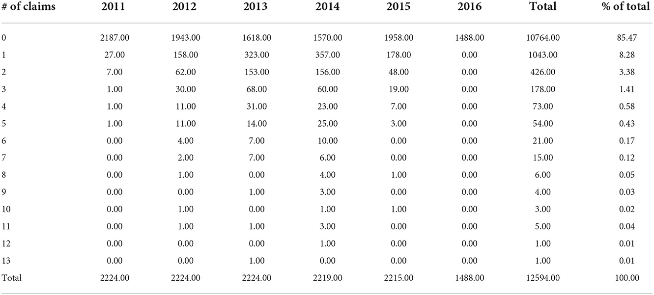
Table 1. Number and percentage of claims, by count and year for the 2011 cohort.
According to the table, the majority of policies had no claims for the duration of the coverage. The data set also shows an extreme number of claims such as 13 claims in the year 2013. However, we did not do any outlier treatment to our data set. Summary statistics for severity per claim for a given year are given in Table 2. It should be noted that the deductible amount was not recorded for almost 99% of policies. Therefore, severities are actually payments made by the insurance company instead of actual losses. However, we do not think that this would impact our findings in this article. The data set is not complete for the year 2016, since there are no claims recorded for the year 2016. We do not believe that there were no claims in the year 2016 but rather the data set does not contain complete information for the year 2016. Thus, we do not plan to use the year 2016 data in our model. Also, the year 2015 excluded about 32.79% of the policies expired before the end of the year. Thus, we used years 2011–2013 for training purposes and year 2014 for testing our models. Our valuation date is 31 December 2013. On the valuation date, we have several previous years' data to train our model. One approach would be to use all previous years' data to train the model. Another approach would be just to use the last year (year 2013) data to train the model. For the random effect model, XGboost model, and random forest model, we used 2011–2013 as the training data set. For the alternative statistical model, we used only 2013 data as the training data. The test data set is always the year 2014.
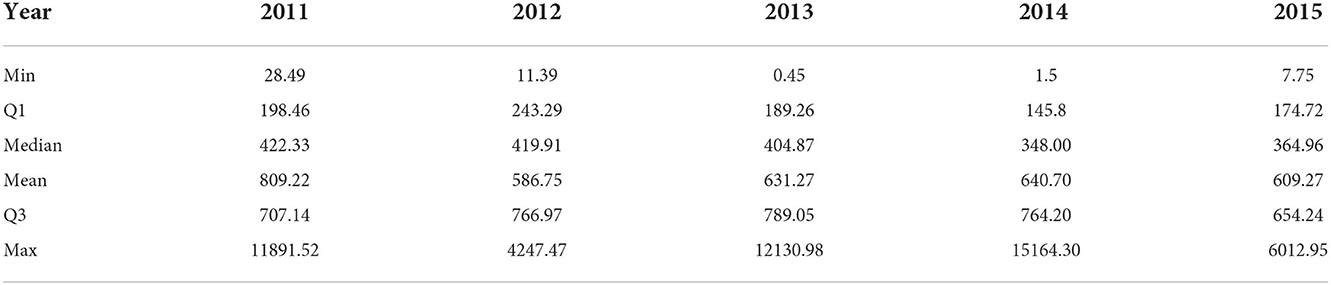
Table 2. Summary statistics of severities per claim for 2011–2014 for the 2011 cohort.
The data set contains other information such as brand, model, generation, vehicle build date, warranty start date, warranty end date, vehicle failure date, and many other characteristics. We also engineered a few features such as exposure, age of the vehicle, and annual losses as of the valuation date. Summary statistics for the age of vehicles in the year 2011 cohort as of 31 December 2011 are given in Table 3.

Table 3. Summary of vehicles age as of 31 December 2011 for the 2011 cohort.
The age is calculated using the build date variable and is used as one of the covariates instead of the build date. The average age of vehicles in the portfolio is around 1 year along with a maximum age of 3.95 years as of the 31 December 2011. The summary statistics for exposure by year are given in Figure 1. For 2011, the average exposure is about 0.53. Then, for years 2012–2014, many vehicles had full exposure for the entire year. After that, some coverage expired either due to the cancelation or reaching the 10,000 mileage restriction.
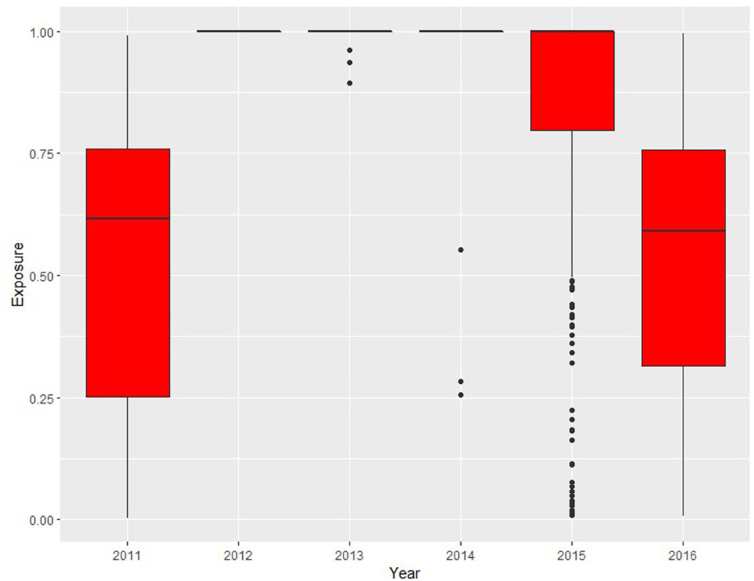
Figure 1. Box plot for coverage exposure by the year.
5. Premium calculation
The data set does not contain the premium related to extended warranty policies. It should be noted that most extended auto warranty policies have a single premium [7]. There are several methods we can employ to get the missing premium for extended warranty policies.
1. Calculate the premium using a past data set.
2. Use a sample of the current data set and calculate the premium based on claims and severities in that sample.
3. Use the premium from another academic research study on extended auto warranty policies.
4. Use online quoted premiums from companies that provide extended warranties.
5. Use the sale price of the vehicle and assume the premium of the extended warranty policy should be equal to a percentage of the sale price.
From these options, we do not have a second data set to calculate the premium. Using the same data set (even with sampling) for calculating the premium may result in premium learning the future severities, thus showing no premium deficiency for the unearned premium risk at the end. We tried to find past research references for the premium on extended auto warranty policies, but could not find a good reference. From the last two options, we decided to use the sale price of the vehicle to calculate the single premium of the extended warranty policy. This approach would give us different premiums for each vehicle. The percentage we used was 2%, which is an ad hoc number. It should be noted that knowledge of the premium is required to calculate PDR but not to evaluate the models itself. We can rewrite observed vs. predicted unearned premium risk models as below :
and
An unearned premium for the kth contract is usually known by the evaluation date. Thus, we think premium itself plays a very little role in the conclusion. The models can be used with different premium amounts, since they do not play any role in the modeling phase. The premium acquisition pattern used in this article is uniform. Under this method, the unearned premium for ith contract on evaluation date E is calculated as
Here ti,E is calculated as the number of days from the warranty start date to the evaluation date E divided by the number of days between the warranty start date and the warranty end date and Pi denotes the single premium paid at the beginning of the ith contract, which is 2% of the sale price of the ith vehicle.
6. Model implementation and results
6.1. Variable description
We considered the following covariates in our analysis: ID, BRAND, MODEL, GENID, TYPE, M, SALE_PRICE, PLANT_ID, CID, STATE, DEDUCTIBLE, USAGE, TOTALPD, AGE, EXPO, and COUNT. The variable ID is the unique identification number of the vehicle/policy. BRAND and MODEL refer to the brand and model of the vehicle. There were three brands and 252 models in the data set. GENID refers to the generation of the vehicle with 28 generations. TYPE is the type of vehicle for license/certification requirement which constitutes five categories. M is a classification of vehicle by a technical component with 18 categories. SALE_PRICE refers to the sale price of the vehicle. PLANT_ID refers to where the vehicle was built with seven categories. CID lists the customer identification number. Some customers may have bought more than one vehicle. There are 1,504 different categories for this variable. STATE refers to the state where the vehicle is located. Each state in North America is given a unique state number with 54 categories in the data set. The DEDUCTIBLE variable refers to the deductible amount. USAGE categorizes vehicles according to industrial classifications. There were 326 categories for this variable in the data set. TOTALPD is the total payment after deductible under the extended warranty contracts. AGE refers to the age of the vehicle, EXPO refers to the exposure of the vehicle for that year, and COUNT refers to the number of claims for that year.
Our intention is to predict PDR for the unearned premium risk for the year 2014. For each model, a subset of variables is used as appropriate. Note that many variables are constant over years such as BRAND, MODEL, GENID, etc. The variable DEDUCTIBLE was not used in the analysis since it was missing in more than 99% of policy records.
6.2. Statistical model
For statistical models, multicollinearity among predictors results in hard to interpret, less stable, and over-fitting models. Therefore, we tested multicollinearity among predictors using R2, Cramer V statistics and the generalized variance inflation factor [27]. Since many variables are the same across years in our data set, auto-correlation is present. The correlation matrix for quantitative variables in training data sets is shown in Table 4.
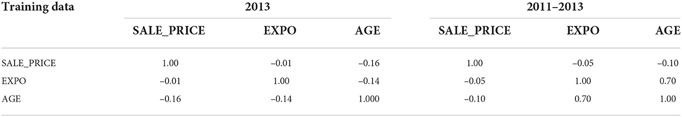
Table 4. Correlation matrix for SALE_PRICE, EXPO, and AGE for training data sets.
6.2.1. Frequency model fitting
We used the HPGENSELECT procedure in SAS 9.4 [28] software with backward selection method and AIC as the criteria to select the best model for the frequency component of the alternative model (negative binomial). Initially, we used the following independent variables in the full model: AGE, SALE_PRICE, BRAND, MODEL, GENID, TYPE, M,PLANT_ID, STATE, CNTRY, and USAGE. The dependent variable is COUNT. The selected model contains AGE, MODEL, and STATE as independent variables. Next we check the collinearity between the MODEL and the BRAND variables using Cramer V statistics and generalized variance inflation factor. The Cramer V Statistic is 1 and the generalized variance inflation factor could not be calculated since BRAND and MODEL are perfectly correlated. Hence strong collinearity exists among the two variables. Given that the Model contains 252 levels and BRAND contains only three levels, we decided to replace MODEL with BRAND to ease interpretation. This results in selected covariates for the frequency model as AGE, BRAND, and STATE. We used the same variables as fixed effects along with ID as a random effect in a random effect Poisson model. Models were implemented in R Core Team [29] using the gamlss, lme4, and glmmTMB packages. Observe that BRAND and STATE variables are constant over the years for each policy, and only age and exposure change over the time. Predictions for each model with Pearson chi-square goodness of fit statistics are shown in Table 5.
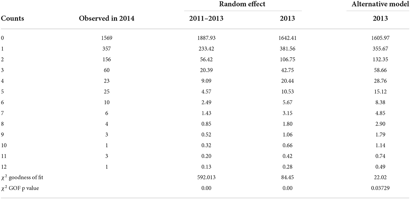
Table 5. Expected frequency for the year 2014 based on two frequency models for training data sets.
The fitted models for the year 2014 are given in Figure 2. Surprisingly, a random effect Poisson model did not perform better than the traditional negative binomial model. According to Figure 2, when the 2011–2013 data were used for training, the random effect model predicted more zero claims than observed. Also observe that the main difference between each model occurred when predicting zero and one claim. Prediction for other numbers of claims looks close enough.
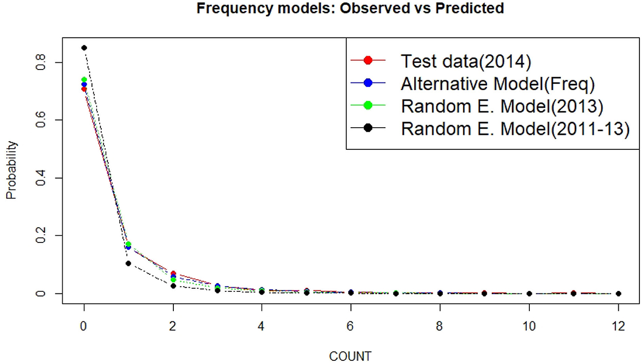
Figure 2. Fitted frequency models for the year 2014 based on two training data sets (2013 vs. 2011–2013) and two models (alternative model vs. random effect Poisson model).
6.2.2. Severity model fitting
For severity modeling without random effect, we used the glm function in R and a stepwise selection method to choose the best model. Initially, we used COUNT, AGE, SALE_PRICE, BRAND, MODEL, GENID, TYPE, M, PLANT_ID, STATE, CNTRY, and USAGE as independent variables. The dependent variable was log(TOTALPD). Then using AIC information criteria, forward and backward step-wise regression methods, we chose COUNT, MODEL, USAGE, and AGE variables for severity modeling. We replaced MODEL with BRAND due to the strong correlation between BRAND and MODEL as well as fewer levels in the BRAND variable. This resulted in COUNT, BRAND, USAGE, and AGE as covariates for severity modeling. The same variables, except COUNT, were used for the severity component of the random effect model. The correlation between COUNT and AGE was negligible. When fitted, the coefficient of the COUNT variable in the severity component of the alternative model is −0.000745. Thus, frequency is not an important predictor for severity prediction in the alternative model. The predicted annual loss for the year 2014 is given by
for the policies in-force as of the evaluation date under each model given in Table 6.

Table 6. Actual and predicted annual total losses for the year 2014 for all policies in-force at 31 December 2013 evaluation date under each model.
The average loss size and the standard deviation per policy are given in Table 7.
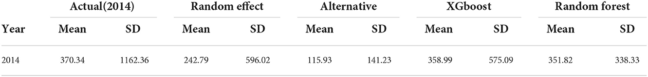
Table 7. Actual and predicted average total annual losses per policy as of the evaluation date.
Mean squared error(MSE), root mean squared error(RMSE), normalized root mean squared error by mean (NRMSE by mean), mean absolute error (MAE), and R2 for the predicted annual losses vs. actual losses are given in Table 8.
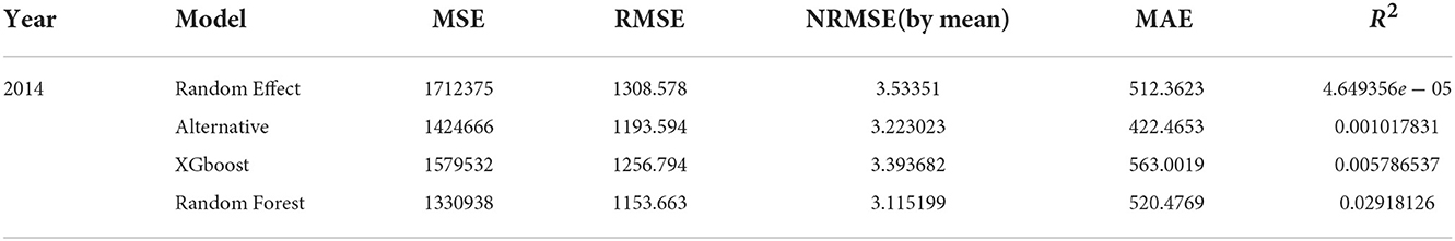
Table 8. Fit statistics for each model.
Finally, we predict the PDR for the unearned premium risk for the year 2014 under each model. The deficiency is indicated by the positive values and a surplus is denoted by the negative values. The reserves are calculated under three metrics: mean, value at risk, and conditional tail expectation. Table 9 summarizes these result. The 95% confidence intervals for the difference between true annual losses against predicted annual losses from the alternative model and the random effect model are given by (205.8386, 302.9774), (73.29819, 181.78059), respectively. Even though none of the statistical models come close to the actual values (or contains zero in confidence interval for differences), we can see that the random effect model is better than the alternative model. This is validated by values in Tables 6, 7, 9.
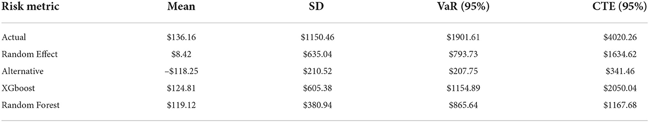
Table 9. Premium deficiency for unearned premium risk under each model.
6.3. XGboost model
The XGboost model can be used for regression and classification. Instead of modeling frequency and severity separately, we used the annual loss for each policy in the training data set to predict the annual loss for each policy in the test data set. We created a new feature named ANNUAL_LOSS by summing up all claim severities for that particular year. Then, we used years 2011–2013 annual losses for training purposes and the year 2014 annual losses for testing purposes. The model was implemented in R using the xgboost package. The hyper-parameters used in the model are given in Table 10.
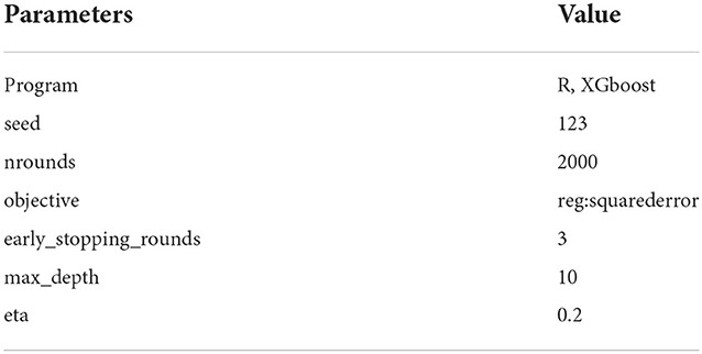
Table 10. Parameters used in the XGboost model.
For XGboost, we choose to consider the BRAND, MODEL, GENID, TYPE, M, SALE_PRICE, STATE, USAGE, EXPO, and AGE. The target variable is ANNUAL_LOSS. The model is evaluated by referring to MSE, RMSE, NRMSE by mean, MAE, R2, and the calculated values are given in Table 8. The predicted annual total loss for the entire cohort, average total loss per policy, and standard deviation of average total loss per policy is shown in Tables 6, 7. Risk metrics for the unearned premium risk under the XGboost model are calculated and are shown in Table 9. The residual plot for the XGboost model on the test data set is shown in Figure 3.
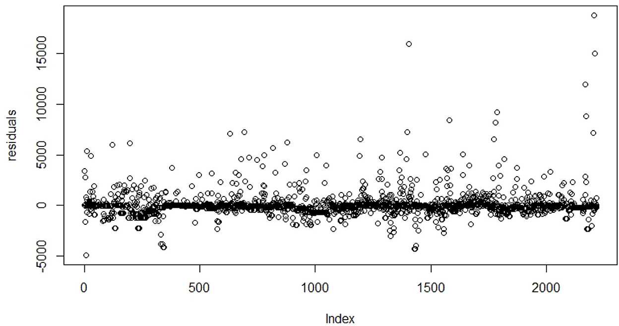
Figure 3. Residual plot for predicted value on test data set under XGboost.
6.4. Random forest model
As an important machine learning method, the random forest can also be used to fit classification and regression models. We used the same variable set we used in the XGboost model and the model was implemented in R Core Team [29] using RandomForest package. The number of trees used in modeling was 500 and the best number of random variables used in each tree, mtry was 42. It should be noted that XGboost and random forest both have common variables for the first 20 most important variables as shown in Table 11. The model fit statistics is shown in Table 8. Predicted total annual losses for year 2014, as well as the average loss per policy and the standard deviation of loss per policy, are shown in Tables 6, 7. The prediction for policies in-force as of the evaluation date: 31 December 2013.
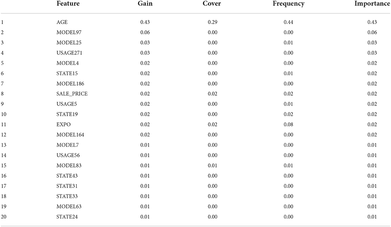
Table 11. Variable importance for the XGboost model.
7. Discussion and conclusion
The purpose of this article is to demonstrate machine learning approaches to calculate premium deficiency risk for an unearned premium. Based on the number of available research articles, we think that the unearned premium risk has attracted less attention from the actuarial community compared to classical claim liability reserves such as IBNR and RBNS. However, the unearned premium risk comprises a major component of premium liability. Therefore, there exist specific guidelines by regulators to monitor the risk everywhere around the world. The existing few research articles on an unearned premium risk mainly utilize traditional statistical models. Also, many make major assumptions regarding the number of claims and the severity. For example, Jessup et al. [9] assumed that the policy can incur only one future loss per given year in their non-homogeneous loss model for unearned premium risk. Another traditional assumption many used in loss modeling is independence between the number of losses and the severity of the loss.
In this article, we were allowed more than one loss per year and dependence between the number of losses and the severity of losses. To benchmark our work, we first developed two statistical models. One was constructed using a random effect model and the other was using a model described by Frees et al. [16]. Both models allowed severity to be conditional on the number of claims. The random effect model took the heterogeneity among policy holders as the random effect. Once we developed these models, we turned our attention to machine learning models. We used two popular machine learning models: XGboost and random forest in this article.
The data set we used in this article is a cohort of extended warranty contracts written in the year 2011. The contracts were written for 60 months. However, we used only years 2011–2013 for training and the year 2014 for testing. We used the only year 2013 as the training data set for the alternative statistical model. The data set contained the number of claims as well as the severity per claim. However, the data set did not contain the actual single premium paid by the policy holder for the warranty contracts. Therefore, we used 2% of the sale price of the vehicle as the single premium of the warranty contract. We acknowledge this is an ad hoc number; however, the premium obtained this way was applied in calculating actual reserve as well as predicted reserve, thus minimizing the effect. We assumed the premium acquisition pattern to be uniform, which can be relaxed very easily without major modification to the models used in the article. According to Table 8, the mean squared error is highest for the random effect model and the lowest for the random forest model. Mean absolute error was the lowest for the alternative statistical model and the highest for the XGboost model. However, when compared with the predicted annual losses for the entire cohort against actual losses for the year 2014, XGboost and random forest models perform very well compared to statistical models. Also, the average loss per policy is more closely predicted by the XGboost model and the random forest model. However, it should be noted that all models under-evaluate actual losses. The same phenomenon happened with the dependent models developed in Jessup et al. [9].
We observed the average actual loss reserve is $136.16 per policy for the year 2014, thus indicating premium deficiency. When we tried to predict using the statistical model, the alternative model predicted –$118.25 per policy or surplus and random effect model predicted a shortage of mere $8.42 per policy. Thus, the difference of $127.74 per policy if the random effect model is used for reserving. Machine learning models predicted $124.81 and $119.12, respectively, which is close to the actual shortage per policy. However, we acknowledge that all model predictions are undervalued compared to real deficiency. Since the sample size (2, 219) for the year 2014 is large, we conducted a simple two-sample t-tests to see whether predicted means for premium deficiencies are different from the true mean. Test statistics for this test can be calculated from values given in Table 9. The test shows that under 0.001, XGboost and random forest models predicted that average premium deficiency is same as the true premium deficiency. Also, both statistical models were rejected under a 0.001 significance level.
The average as a risk measure may not be suitable for reserving purposes. Many use value at risk (VaR) or tail value at risk (TVaR) as the risk measure for this purpose. Under VaR and TVaR, for a 95% confidence, the XGboost model predictions are the closest to actual values. When we used statistical models, the difference was much larger. The same phenomena can be seen in previous research. For example, Table 5 in the article [9] showed that the observed reserve is –8,247,000 and the predicted mean reserve of –4,302,000 and –2,284,000 for independent models. For the year 2014, the distribution of the unearned premium risk is given in Figure 4.
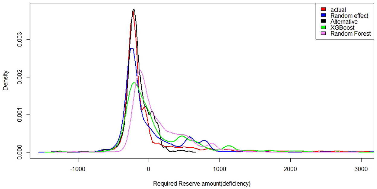
Figure 4. Reserve amount for the unearned premium risk under each model for test data set.
According to the density plot, the alternative statistical model density curve closely follows the actual reserve density curve when the required reserve amount is zero or negative (surplus). The density curve shows a lighter tail to the right for the alternative model compared with the actual curve. However, XGboost and Random forest models show thick tails to the right, thus capturing extreme values and hence predicting reserves more correctly.
We have shown that ML techniques can be used in place of the statistical model or at least supplement results on calculating unearned premium risk and required deficiency reserves. Our calculations show that ML models predict deficiency reserves more closely than the two statistical models we used in this article. We should consider using more ML techniques. For example, deep learning techniques should be considered and compared with traditional models for unearned premium risks. We assumed a uniform acquisition pattern for premium. This can be relaxed since companies need to decide how to divide premiums as earned vs. unearned at the beginning for bookkeeping purposes. Once the rule is available, the unearned premium at each valuation date is known in advance. We did not consider seasonality and the time of loss in our analysis. In statistical models, for the given observational unit {it}, the intensity function only vary with covariates xit. However, relaxing this assumption and allowing the intensity function to depend on the time of the year as well as covariates can bring seasonality to the model. Further research should be carried out in this aspect.
Data availability statement
The datasets presented in this article are not readily available because data is confidential. Not available to public. Requests to access the datasets should be directed to vmanathunga@mtsu.edu.
Author contributions
All authors listed have made a substantial, direct, and intellectual contribution to the work and approved it for publication.
Conflict of interest
The authors declare that the research was conducted in the absence of any commercial or financial relationships that could be construed as a potential conflict of interest.
Publisher's note
All claims expressed in this article are solely those of the authors and do not necessarily represent those of their affiliated organizations, or those of the publisher, the editors and the reviewers. Any product that may be evaluated in this article, or claim that may be made by its manufacturer, is not guaranteed or endorsed by the publisher.
References
1. SOA. Earned Premium, Society of Actuaries. (2022). Available online at: https://actuarialtoolkit.soa.org/tool/glossary/earned-premium (accessed on August 16, 2022).
2. SOA. Unearned Premium, Society of Actuaries. (2022). Available online at: https://actuarialtoolkit.soa.org/tool/glossary/unearned-premiums (accessed on August 16, 2022).
3. Bornhuetter RL, Ferguson RE. The actuary and IBNR. In: Proceedings of the Casualty Actuarial Society. Vol. 59–112. (1972). p. 181–95.
4. Mack T. Distribution-free calculation of the standard error of chain ladder reserve estimates. ASTIN Bull J IAA. (1993) 23:213–25. doi: 10.2143/AST.23.2.2005092
5. Schmidt KD. A Bibliography on Loss Reserving. (2011). Available online at: https://tu-dresden.de/mn/math/stochastik/ressourcen/dateien/schmidt/dsvm/reserve.pdf?lang=en (accessed September 15, 2022).
6. Cantin C, Trahan P. A study note on the actuarial evaluation of premium liabilities. J Actuarial Pract. (1999) 7:5–72.
8. Cheng J. Unearned premiums and deferred policy acquisition expenses in automobile extended warranty insurance. J Actuarial Pract. (2002) 10:63–95. Available online at: https://digitalcommons.unl.edu/joap/41/
9. Jessup S, Boucher JP, Pigeon M. On fitting dependent nonhomogeneous loss models to unearned premium risk. North Am Actuarial J. (2021) 25:524–42. doi: 10.1080/10920277.2020.1776623
10. Klugman SA, Panjer HH, Willmot GE. Loss Models: From Data to Decisions. John Wiley & Sons (2019).
11. Richman R. AI in actuarial science-a review of recent advances-part 1. Ann Actuarial Sci. (2021) 15:207–29. doi: 10.1017/S1748499520000238
12. Richman R. AI in actuarial science-a review of recent advances-part 2. Ann Actuarial Sci. (2021) 15:230–58. doi: 10.1017/S174849952000024X
13. Ly A, Uthayasooriyar B, Wang T. A survey on natural language processing (nlp) and applications in insurance. arXiv preprint arXiv:201000462. (2020). doi: 10.48550/arXiv.2010.00462
14. Xu S, Zhang C, Hong D. BERT-based NLP techniques for classification and severity modeling in basic warranty data study. Insurance. (2022) 107:57–67. doi: 10.1016/j.insmatheco.2022.07.013
15. Krishnan M. Against interpretability: a critical examination of the interpretability problem in machine learning. Philos Technol. (2020) 33:487–502. doi: 10.1007/s13347-019-00372-9
16. Frees EW, Gao J, Rosenberg MA. Predicting the frequency and amount of health care expenditures. North Am Actuarial J. (2011) 15:377–92. doi: 10.1080/10920277.2011.10597626
17. PavloviĆ B. Unexpired risk reserve. In: Kocovic J, Jovanovic Gavrilovic B, Jakovcevic D, editors. Achieved Results and Prospects of Insurance Market Development in Modern World. Belgrade: Faculty of Economics, Publishing Centre (2012). p. 279–93.
18. NAIC. Statutory Issue Paper No. 65, The National Association of Insurance Commissioners. (1998). Available online at: https://content.naic.org/sites/default/files/inline-files/053-O.pdf (accessed August 16, 2022).
19. NAIC. Official NAIC Annual Statement Instructions- Property/Casualty-For the 2020 reporting year -Adopted by the NAIC as of June 2020. The National Association of Insurance Commissioners (2020). Available online at: https://www.in.gov/idoi/files/2020_ASI_PC.pdf (accessed August 16, 2022).
20. Lusk VS,. Unearned Premium Reserve for Long-Term Policies. (2005). Available online at: https://www.casact.org/pubs/forum/99fforum/99ff215.pdf (accessed August 16, 2022).
21. NAIC. Statutory Issue Paper No. 53, The National Association of Insurance Commissioners. (1998). Available online at: https://content.naic.org/sites/default/files/inline-files/065_j.pdf (accessed August 16, 2022).
22. Shi P, Valdez EA. Longitudinal modeling of insurance claim counts using jitters. Scand Actuar J. (2014) 2014:159–79. doi: 10.1080/03461238.2012.670611
23. Yirga AA, Melesse SF, Mwambi HG, Ayele DG. Negative binomial mixed models for analyzing longitudinal CD4 count data. Sci Rep. (2020) 10:1–5. doi: 10.1038/s41598-020-73883-7
24. Frees EW, Valdez EA. Hierarchical insurance claims modeling. J Am Stat Assoc. (2008) 103:1457–69. doi: 10.1198/016214508000000823
25. Chen T, He T, Benesty M, Khotilovich V, Tang Y, Cho H, et al. Xgboost: extreme gradient boosting. R package version 04-2 (2015).
26. Hastie T, Tibshirani R, Friedman JH, Friedman JH. The Elements of Statistical Learning: Data Mining, Inference, and Prediction. Vol. 2. Springer (2009).
27. Fox J, Monette G. Generalized collinearity diagnostics. J Am Stat Assoc. (1992) 87:178–83. doi: 10.1080/01621459.1992.10475190
28. SAS Institiute,. The Output Was Generated Using SAS 9.4 Software. Cary, NC: Copyright ©SAS Institute Inc. SAS all other SAS Institute Inc. product or service names are registered trademarks or trademarks of SAS Institute Inc. (2022). Available from: Available online at: https://www.sas.com/en_us/home.html
29. R Core Team,. R: A Language Environment for Statistical Computing. Vienna: R Core Team (2021). Available online at: https://www.R-project.org/
Keywords: unearned premium risk, random effect models, XGBoost method, random forest, extended auto warranty
Citation: Manathunga V and Zhu D (2022) Unearned premium risk and machine learning techniques. Front. Appl. Math. Stat. 8:1056529. doi: 10.3389/fams.2022.1056529
Received: 28 September 2022; Accepted: 08 November 2022;
Published: 01 December 2022.
Edited by:
Tianxiang Shi, Temple University, United StatesReviewed by:
Diganta Mukherjee, Indian Statistical Institute, IndiaGuojun Gan, University of Connecticut, United States
Copyright © 2022 Manathunga and Zhu. This is an open-access article distributed under the terms of the Creative Commons Attribution License (CC BY). The use, distribution or reproduction in other forums is permitted, provided the original author(s) and the copyright owner(s) are credited and that the original publication in this journal is cited, in accordance with accepted academic practice. No use, distribution or reproduction is permitted which does not comply with these terms.
*Correspondence: Vajira Manathunga, vajira.manathunga@mtsu.edu